AboutHap

About HAP: Simplicial and cubical complexes

1. Simplicial Complexes

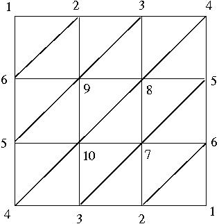
A finite simplicial complex can be created in HAP by specifying its maximal simplices. For instance, the following commmands construct the simplicial projective plane

and then calculate its integral homologies from the associated cellular chain complex.

gap> L:=[[1,2,6],[2,6,9],[2,3,9],[3,8,9],[3,4,8],[4,5,8],
> [5,6,9],[5,9,10],[8,9,10],[7,8,10],[5,7,8],[5,6,7],
> [4,5,10],[3,4,10],[3,7,10],[2,3,7],[2,6,7],[1,2,6]];;

gap> ProjPlane:=MaximalSimplicesToSimplicialComplex(L);
Simplicial complex of dimension 2.

gap> C:=ChainComplex(ProjPlane);
Chain complex of length 2 in characteristic 0 .

gap> Homology(C,0);
[ 0 ]
gap> Homology(C,1);
[ 2 ]
gap> Homology(C,2);
[ ]

The following commands compute the low-dimensional integral homologies of a 10-dimensional simplicial sphere.

gap> n:=10;;
gap> n_Sphere:=MaximalSimplicesToSimplicialComplex(Combinations([0..n+1],n+1));
Simplicial complex of dimension 10.

gap> C:=ChainComplex(n_Sphere);
Chain complex of length 10 in characteristic 0 .

gap> List([0..n],m->Homology(C,m));
[ [ 0 ], [ ], [ ], [ ], [ ], [ ], [ ], [ ], [ ], [ ], [ 0 ], [ ] ]

The simplicial complex arising as the order complex of the poset of non-trivial elementary abelian p-subgroups of a finite group G has been studied by D. Quillen and others. The following commands contruct this simplicial complex for the Sylow 2-subgroup of the Mathieu group M₁₂ (with p=2), and then verify that in this case the simplicial complex is contractible.

gap> Q:=QuillenComplex(SylowSubgroup(MathieuGroup(12),2),2);
Simplicial complex of dimension 2.

gap> C:=ChainComplex(Q);
Chain complex of length 2 in characteristic 0 .

gap> Homology(C,0);
[ 0 ]
gap> Homology(C,1);
[ ]
gap> Homology(C,2);
[ ]

2. Cubical Complexes

In HAP we us the term "pure cubical complex" to mean a subspace of d-dimensional euclidian space arising as a union of finitely many d-dimensional unit cubes whose vertices have integral coordinates. A pure cubical space can be created by specifying a d-dimensional array of 0s and 1s. For instance, the following commands construct a 3-dimensional cubical 2-sphere and verify its homology in low dimensions.

gap> a:=[[1,1,1],[1,1,1],[1,1,1]];;
gap> b:=[[1,1,1],[1,0,1],[1,1,1]];;
gap> c:=[[1,1,1],[1,1,1],[1,1,1]];;
gap> array:=[a,b,c];;
gap> 2_sphere:=PureCubicalComplex(array);
Pure cubical complex of dimension 3.

gap> C:=ChainComplex(2_sphere);
Chain complex of length 3 in characteristic 0 .

gap> Homology(C,0);
[ 0 ]
gap> Homology(C,1);
[ ]
gap> Homology(C,2);
[ 0 ]
gap> Homology(C,3);
[ ]

The Cech complex of a pure cubical complex is a simplicial complex such that the geometric realizations of the two complexes are homotopy equivalent. The following commands compute the Cech complex of the cubical 2-sphere and (again) verify the low dimensional homology of the 2-sphere.

gap> S:=CechComplexOfPureCubicalComplex(2_sphere);
Simplicial complex of dimension 3.

gap> C:=ChainComplex(S);
Chain complex of length 3 in characteristic 0 .

gap> Homology(C,0);
[ 0 ]
gap> Homology(C,1);
[ ]
gap> Homology(C,2);
[ 0 ]
gap> Homology(C,3);
[ ]

The above cubical 2-sphere has twenty-six 3-cells. The following commands compute a homotopy retract with just six 3-cells.

gap> new_sphere:=ContractedComplex(2_sphere);
Pure cubical complex of dimension 3.

gap> C:=ChainComplex(2_sphere);;
gap> D:=ChainComplex(new_sphere);;
gap> C!.dimension(3);
26
gap> D!.dimension(3);
6

The following command shows that the Cech complex of this smaller 3-dimensional 2-sphere is actually a 2-dimensional simplicial complex.

gap> S:=CechComplexOfPureCubicalComplex(new_sphere);
Simplicial complex of dimension 2.

The following commands compute a 3-dimensional simplicial complex which is homotopic to a torus.

gap> Circle:=PureCubicalComplex([[1,1,1],[1,0,1],[1,1,1]]);
Pure cubical complex of dimension 2.

gap> Torus:=DirectProductOfPureCubicalComplexes(Circle,Circle);
Pure cubical complex of dimension 4.

gap> ContractPureCubicalComplex(Torus);;

gap> SimplicialTorus:=CechComplexOfPureCubicalComplex(Torus);
Simplicial complex of dimension 3.

A digital photograph can be represented as a 2-dimensional pure cubical complex. This is done by choosing an integer threshold and including a 2-cell in the pure cubical complex for each pixel where the sum of the three RGB values iis less than the threshold.

The following commands use a threshold of 400 to represent the image

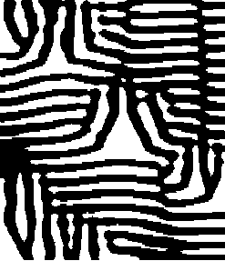
as a pure cubical complex. The complex has 40949 2-dimensional cells.

gap> image:=ReadImageAsPureCubicalComplex("bw_image.bmp",400);
Pure cubical complex of dimension 2.

gap> C:=ChainComplex(image);
Chain complex of length 2 in characteristic 0 .

gap> C!.dimension(0);
45664
gap> C!.dimension(1);
86630
gap> C!.dimension(2);
40949

The number of cells in the above cubical complex makes it difficult to compute the homology of the associated cellular chain complex. One way around the difficulty is to:

Find a homotopy retract R of the pure cubical complex.
Find a large contractible subcomplex S in R.
Construct the quotient C(R)/C(S) of the cellular chain complexes.
Use the fact that H_n(R) = H_n( C(R)/C(S) ) for n>0 and that H₀(R) is isomorphic to the direct sum H₀(C(R)/C(S))+H₀(S).

The following commands apply Steps 1-4 in order to calculate that the above image has 3 path components and 20 1-cycles.

gap> image:=ReadImageAsPureCubicalComplex("bw_image.bmp",400);
Pure cubical complex of dimension 2.

gap> R:=ContractedComplex(image);
Pure cubical complex of dimension 2.

gap> S:=ContractibleSubcomplexOfPureCubicalComplex(R);
Pure cubical complex of dimension 2.

gap> C:=ChainComplexOfPair(R,S);
Chain complex of length 2 in characteristic 0 .

gap> Homology(C,0);
[ 0, 0 ]

gap> Homology(C,1);
[ 0, 0, 0, 0, 0, 0, 0, 0, 0, 0, 0, 0, 0, 0, 0, 0, 0, 0, 0, 0 ]

Contents