Navigation
- index
- modules |
- next |
- previous |
- Graph Theory »

All graphs in Sage can be built through the graphs object. In order to build a complete graph on 15 elements, one can do:
sage: g = graphs.CompleteGraph(15)
To get a path with 4 vertices, and the house graph:
sage: p = graphs.PathGraph(4)
sage: h = graphs.HouseGraph()
More interestingly, one can get the list of all graphs that Sage knows how to build by typing graphs. in Sage and then hitting tab.
Basic structures
Small Graphs
A small graph is just a single graph and has no parameter influencing the number of edges or vertices.
Platonic solids (ordered ascending by number of vertices)
| TetrahedralGraph | HexahedralGraph | DodecahedralGraph |
| OctahedralGraph | IcosahedralGraph |
Families of graphs
A family of graph is an infinite set of graphs which can be indexed by fixed number of parameters, e.g. two integer parameters. (A method whose name starts with a small letter does not return a single graph object but a graph iterator or a list of graphs or ...)
Chessboard Graphs
| BishopGraph | KnightGraph | RookGraph |
| KingGraph | QueenGraph |
Intersection graphs
These graphs are generated by geometric representations. The objects of the representation correspond to the graph vertices and the intersections of objects yield the graph edges.
| IntersectionGraph | OrthogonalArrayBlockGraph | ToleranceGraph |
| IntervalGraph | PermutationGraph |
Random graphs
Graphs with a given degree sequence
| DegreeSequence | DegreeSequenceConfigurationModel | DegreeSequenceTree |
| DegreeSequenceBipartite | DegreeSequenceExpected |
Miscellaneous
| WorldMap |
AUTHORS:
A class consisting of constructors for several common graphs, as well as orderly generation of isomorphism class representatives. See the module's help for a list of supported constructors.
A list of all graphs and graph structures (other than isomorphism class representatives) in this database is available via tab completion. Type “graphs.” and then hit the tab key to see which graphs are available.
The docstrings include educational information about each named graph with the hopes that this class can be used as a reference.
For all the constructors in this class (except the octahedral, dodecahedral, random and empty graphs), the position dictionary is filled to override the spring-layout algorithm.
ORDERLY GENERATION:
graphs(vertices, property=lambda x: True, augment='edges', size=None)
This syntax accesses the generator of isomorphism class representatives. Iterates over distinct, exhaustive representatives.
Also: see the use of the optional nauty package for generating graphs at the nauty_geng() method.
INPUT:
EXAMPLES:
Print graphs on 3 or less vertices:
sage: for G in graphs(3, augment='vertices'):
...    print G
Graph on 0 vertices
Graph on 1 vertex
Graph on 2 vertices
Graph on 3 vertices
Graph on 3 vertices
Graph on 3 vertices
Graph on 2 vertices
Graph on 3 vertices
Note that we can also get graphs with underlying Cython implementation:
sage: for G in graphs(3, augment='vertices', implementation='c_graph'):
...    print G
Graph on 0 vertices
Graph on 1 vertex
Graph on 2 vertices
Graph on 3 vertices
Graph on 3 vertices
Graph on 3 vertices
Graph on 2 vertices
Graph on 3 vertices
Print graphs on 3 vertices.
sage: for G in graphs(3):
...    print G
Graph on 3 vertices
Graph on 3 vertices
Graph on 3 vertices
Graph on 3 vertices
Generate all graphs with 5 vertices and 4 edges.
sage: L = graphs(5, size=4)
sage: len(list(L))
6
Generate all graphs with 5 vertices and up to 4 edges.
sage: L = list(graphs(5, lambda G: G.size() <= 4))
sage: len(L)
14
sage: graphs_list.show_graphs(L) # long time
Generate all graphs with up to 5 vertices and up to 4 edges.
sage: L = list(graphs(5, lambda G: G.size() <= 4, augment='vertices'))
sage: len(L)
31
sage: graphs_list.show_graphs(L)              # long time
Generate all graphs with degree at most 2, up to 6 vertices.
sage: property = lambda G: ( max([G.degree(v) for v in G] + [0]) <= 2 )
sage: L = list(graphs(6, property, augment='vertices'))
sage: len(L)
45
Generate all bipartite graphs on up to 7 vertices: (see OEIS sequence A033995)
sage: L = list( graphs(7, lambda G: G.is_bipartite(), augment='vertices') )
sage: [len([g for g in L if g.order() == i]) for i in [1..7]]
[1, 2, 3, 7, 13, 35, 88]
Generate all bipartite graphs on exactly 7 vertices:
sage: L = list( graphs(7, lambda G: G.is_bipartite()) )
sage: len(L)
88
Generate all bipartite graphs on exactly 8 vertices:
sage: L = list( graphs(8, lambda G: G.is_bipartite()) ) # long time
sage: len(L)                                            # long time
303
Remember that the property argument does not behave as a filter, except for appropriately inheritable properties:
sage: property = lambda G: G.is_vertex_transitive()
sage: len(list(graphs(4, property)))
1
sage: len(filter(property, graphs(4)))
4
sage: property = lambda G: G.is_bipartite()
sage: len(list(graphs(4, property)))
7
sage: len(filter(property, graphs(4)))
7
Generate graphs on the fly: (see OEIS sequence A000088)
sage: for i in range(0, 7):
...    print len(list(graphs(i)))
1
1
2
4
11
34
156
Generate all simple graphs, allowing loops: (see OEIS sequence A000666)
sage: L = list(graphs(5,augment='vertices',loops=True))               # long time
sage: for i in [0..5]: print i, len([g for g in L if g.order() == i]) # long time
0 1
1 2
2 6
3 20
4 90
5 544
Generate all graphs with a specified degree sequence (see OEIS sequence A002851):
sage: for i in [4,6,8]:  # long time (4s on sage.math, 2012)
...       print i, len([g for g in graphs(i, degree_sequence=[3]*i) if g.is_connected()])
4 1
6 2
8 5
sage: for i in [4,6,8]:  # long time (7s on sage.math, 2012)
...       print i, len([g for g in graphs(i, augment='vertices', degree_sequence=[3]*i) if g.is_connected()])
4 1
6 2
8 5
sage: print 10, len([g for g in graphs(10,degree_sequence=[3]*10) if g.is_connected()]) # not tested
10 19
Make sure that the graphs are really independent and the generator survives repeated vertex removal (trac ticket #8458):
sage: for G in graphs(3):
...       G.delete_vertex(0)
...       print(G.order())
2
2
2
2
REFERENCE:
Returns the affine polar graph \(VO^+(d,q),VO^-(d,q)\) or \(VO(d,q)\).
Affine Polar graphs are built from a \(d\)-dimensional vector space over \(F_q\), and a quadratic form which is hyperbolic, elliptic or parabolic according to the value of sign.
Note that \(VO^+(d,q),VO^-(d,q)\) are strongly regular graphs, while \(VO(d,q)\) is not.
For more information on Affine Polar graphs, see Affine Polar Graphs page of Andries Brouwer’s website.
INPUT:
Note
The graph \(VO^\epsilon(d,q)\) is the graph induced by the non-neighbors of a vertex in an Orthogonal Polar Graph \(O^\epsilon(d+2,q)\).
EXAMPLES:
The Brouwer-Haemers graph is isomorphic to \(VO^-(4,3)\):
sage: g = graphs.AffineOrthogonalPolarGraph(4,3,"-")
sage: g.is_isomorphic(graphs.BrouwerHaemersGraph())
True
Some examples from Brouwer’s table or strongly regular graphs:
sage: g = graphs.AffineOrthogonalPolarGraph(6,2,"-"); g
Affine Polar Graph VO^-(6,2): Graph on 64 vertices
sage: g.is_strongly_regular(parameters=True)
(64, 27, 10, 12)
sage: g = graphs.AffineOrthogonalPolarGraph(6,2,"+"); g
Affine Polar Graph VO^+(6,2): Graph on 64 vertices
sage: g.is_strongly_regular(parameters=True)
(64, 35, 18, 20)
When sign is None:
sage: g = graphs.AffineOrthogonalPolarGraph(5,2,None); g
Affine Polar Graph VO^-(5,2): Graph on 32 vertices
sage: g.is_strongly_regular(parameters=True)
False
sage: g.is_regular()
True
sage: g.is_vertex_transitive()
True
Returns the Balaban 10-cage.
The Balaban 10-cage is a 3-regular graph with 70 vertices and 105 edges. See its Wikipedia page.
The default embedding gives a deeper understanding of the graph’s automorphism group. It is divided into 4 layers (each layer being a set of points at equal distance from the drawing’s center). From outside to inside:
This graph is not vertex-transitive, and its vertices are partitioned into 3 orbits: L2, L3, and the union of L1 of L4 whose elements are equivalent.
INPUT:
EXAMPLES:
sage: g = graphs.Balaban10Cage()
sage: g.girth()
10
sage: g.chromatic_number()
2
sage: g.diameter()
6
sage: g.is_hamiltonian()
True
sage: g.show(figsize=[10,10])   # long time
TESTS:
sage: graphs.Balaban10Cage(embedding='foo')
Traceback (most recent call last):
...
ValueError: The value of embedding must be 1 or 2.
Returns the Balaban 11-cage.
For more information, see this Wikipedia article on the Balaban 11-cage.
INPUT:
Note
The vertex labeling changes according to the value of embedding=1.
EXAMPLES:
Basic properties:
sage: g = graphs.Balaban11Cage()
sage: g.order()
112
sage: g.size()
168
sage: g.girth()
11
sage: g.diameter()
8
sage: g.automorphism_group().cardinality()
64
Our many embeddings:
sage: g1 = graphs.Balaban11Cage(embedding=1)
sage: g2 = graphs.Balaban11Cage(embedding=2)
sage: g3 = graphs.Balaban11Cage(embedding=3)
sage: g1.show(figsize=[10,10])   # long time
sage: g2.show(figsize=[10,10])   # long time
sage: g3.show(figsize=[10,10])   # long time
Proof that the embeddings are the same graph:
sage: g1.is_isomorphic(g2) # g2 and g3 are obviously isomorphic
True
TESTS:
sage: graphs.Balaban11Cage(embedding='xyzzy')
Traceback (most recent call last):
...
ValueError: The value of embedding must be 1, 2, or 3.
REFERENCES:
| [FAGDC] | Fifth Annual Graph Drawing Contest P. Eaded, J. Marks, P.Mutzel, S. North http://www.merl.com/papers/docs/TR98-16.pdf |
Returns the perfectly balanced tree of height \(h \geq 1\), whose root has degree \(r \geq 2\).
The number of vertices of this graph is \(1 + r + r^2 + \cdots + r^h\), that is, \(\frac{r^{h+1} - 1}{r - 1}\). The number of edges is one less than the number of vertices.
INPUT:
OUTPUT:
The perfectly balanced tree of height \(h \geq 1\) and whose root has degree \(r \geq 2\). A NetworkXError is returned if \(r < 2\) or \(h < 1\).
ALGORITHM:
Uses NetworkX.
EXAMPLES:
A balanced tree whose root node has degree \(r = 2\), and of height \(h = 1\), has order 3 and size 2:
sage: G = graphs.BalancedTree(2, 1); G
Balanced tree: Graph on 3 vertices
sage: G.order(); G.size()
3
2
sage: r = 2; h = 1
sage: v = 1 + r
sage: v; v - 1
3
2
Plot a balanced tree of height 5, whose root node has degree \(r = 3\):
sage: G = graphs.BalancedTree(3, 5)
sage: G.show()   # long time
A tree is bipartite. If its vertex set is finite, then it is planar.
sage: r = randint(2, 5); h = randint(1, 7)
sage: T = graphs.BalancedTree(r, h)
sage: T.is_bipartite()
True
sage: T.is_planar()
True
sage: v = (r^(h + 1) - 1) / (r - 1)
sage: T.order() == v
True
sage: T.size() == v - 1
True
TESTS:
Normally we would only consider balanced trees whose root node has degree \(r \geq 2\), but the construction degenerates gracefully:
sage: graphs.BalancedTree(1, 10)
Balanced tree: Graph on 2 vertices

sage: graphs.BalancedTree(-1, 10)
Balanced tree: Graph on 1 vertex
Similarly, we usually want the tree must have height \(h \geq 1\) but the algorithm also degenerates gracefully here:
sage: graphs.BalancedTree(3, 0)
Balanced tree: Graph on 1 vertex

sage: graphs.BalancedTree(5, -2)
Balanced tree: Graph on 0 vertices

sage: graphs.BalancedTree(-2,-2)
Balanced tree: Graph on 0 vertices
Returns a barbell graph with 2*n1 + n2 nodes. The argument n1 must be greater than or equal to 2.
A barbell graph is a basic structure that consists of a path graph of order n2 connecting two complete graphs of order n1 each.
This constructor depends on NetworkX numeric labels. In this case, the n1-th node connects to the path graph from one complete graph and the n1 + n2 + 1-th node connects to the path graph from the other complete graph.
INPUT:
OUTPUT:
A barbell graph of order 2*n1 + n2. A ValueError is returned if n1 < 2 or n2 < 0.
ALGORITHM:
Uses NetworkX.
PLOTTING:
Upon construction, the position dictionary is filled to override the spring-layout algorithm. By convention, each barbell graph will be displayed with the two complete graphs in the lower-left and upper-right corners, with the path graph connecting diagonally between the two. Thus the n1-th node will be drawn at a 45 degree angle from the horizontal right center of the first complete graph, and the n1 + n2 + 1-th node will be drawn 45 degrees below the left horizontal center of the second complete graph.
EXAMPLES:
Construct and show a barbell graph Bar = 4, Bells = 9:
sage: g = graphs.BarbellGraph(9, 4); g
Barbell graph: Graph on 22 vertices
sage: g.show() # long time
An n1 >= 2, n2 >= 0 barbell graph has order 2*n1 + n2. It has the complete graph on n1 vertices as a subgraph. It also has the path graph on n2 vertices as a subgraph.
sage: n1 = randint(2, 2*10^2)
sage: n2 = randint(0, 2*10^2)
sage: g = graphs.BarbellGraph(n1, n2)
sage: v = 2*n1 + n2
sage: g.order() == v
True
sage: K_n1 = graphs.CompleteGraph(n1)
sage: P_n2 = graphs.PathGraph(n2)
sage: s_K = g.subgraph_search(K_n1, induced=True)
sage: s_P = g.subgraph_search(P_n2, induced=True)
sage: K_n1.is_isomorphic(s_K)
True
sage: P_n2.is_isomorphic(s_P)
True
Create several barbell graphs in a Sage graphics array:
sage: g = []
sage: j = []
sage: for i in range(6):
...       k = graphs.BarbellGraph(i + 2, 4)
...       g.append(k)
...
sage: for i in range(2):
...       n = []
...       for m in range(3):
...           n.append(g[3*i + m].plot(vertex_size=50, vertex_labels=False))
...       j.append(n)
...
sage: G = sage.plot.graphics.GraphicsArray(j)
sage: G.show() # long time
TESTS:
The input n1 must be \(\geq 2\):
sage: graphs.BarbellGraph(1, randint(0, 10^6))
Traceback (most recent call last):
...
ValueError: Invalid graph description, n1 should be >= 2
sage: graphs.BarbellGraph(randint(-10^6, 1), randint(0, 10^6))
Traceback (most recent call last):
...
ValueError: Invalid graph description, n1 should be >= 2
The input n2 must be \(\geq 0\):
sage: graphs.BarbellGraph(randint(2, 10^6), -1)
Traceback (most recent call last):
...
ValueError: Invalid graph description, n2 should be >= 0
sage: graphs.BarbellGraph(randint(2, 10^6), randint(-10^6, -1))
Traceback (most recent call last):
...
ValueError: Invalid graph description, n2 should be >= 0
sage: graphs.BarbellGraph(randint(-10^6, 1), randint(-10^6, -1))
Traceback (most recent call last):
...
ValueError: Invalid graph description, n1 should be >= 2
Returns the Bidiakis cube.
For more information, see this Wikipedia article on the Bidiakis cube.
EXAMPLES:
The Bidiakis cube is a 3-regular graph having 12 vertices and 18 edges. This means that each vertex has a degree of 3.
sage: g = graphs.BidiakisCube(); g
Bidiakis cube: Graph on 12 vertices
sage: g.show()  # long time
sage: g.order()
12
sage: g.size()
18
sage: g.is_regular(3)
True
It is a Hamiltonian graph with diameter 3 and girth 4:
sage: g.is_hamiltonian()
True
sage: g.diameter()
3
sage: g.girth()
4
It is a planar graph with characteristic polynomial \((x - 3) (x - 2) (x^4) (x + 1) (x + 2) (x^2 + x - 4)^2\) and chromatic number 3:
sage: g.is_planar()
True
sage: bool(g.characteristic_polynomial() == expand((x - 3) * (x - 2) * (x^4) * (x + 1) * (x + 2) * (x^2 + x - 4)^2))
True
sage: g.chromatic_number()
3
Returns the Biggs-Smith graph.
For more information, see this Wikipedia article on the Biggs-Smith graph.
INPUT:
EXAMPLES:
Basic properties:
sage: g = graphs.BiggsSmithGraph()
sage: g.order()
102
sage: g.size()
153
sage: g.girth()
9
sage: g.diameter()
7
sage: g.automorphism_group().cardinality()
2448
sage: g.show(figsize=[10, 10])   # long time
The other embedding:
sage: graphs.BiggsSmithGraph(embedding=2).show()
TESTS:
sage: graphs.BiggsSmithGraph(embedding='xyzzy')
Traceback (most recent call last):
...
ValueError: The value of embedding must be 1 or 2.
Returns the \(d\)-dimensional Bishop Graph with prescribed dimensions.
The 2-dimensional Bishop Graph of parameters \(n\) and \(m\) is a graph with \(nm\) vertices in which each vertex represents a square in an \(n \times m\) chessboard, and each edge corresponds to a legal move by a bishop.
The \(d\)-dimensional Bishop Graph with \(d >= 2\) has for vertex set the cells of a \(d\)-dimensional grid with prescribed dimensions, and each edge corresponds to a legal move by a bishop in any pairs of dimensions.
The Bishop Graph is not connected.
INPUTS:
EXAMPLES:
The (n,m)-Bishop Graph is not connected:
sage: G = graphs.BishopGraph( [3, 4] )
sage: G.is_connected()
False
The Bishop Graph can be obtained from Knight Graphs:
sage: for d in xrange(3,12):   # long time
....:     H = Graph()
....:     for r in xrange(1,d+1):
....:         B = graphs.BishopGraph([d,d],radius=r)
....:         H.add_edges( graphs.KnightGraph([d,d],one=r,two=r).edges() )
....:         if not B.is_isomorphic(H):
....:            print "that's not good!"
Returns the first Blanusa Snark Graph.
The Blanusa graphs are two snarks on 18 vertices and 27 edges. For more information on them, see the Wikipedia article Blanusa_snarks.
See also
EXAMPLES:
sage: g = graphs.BlanusaFirstSnarkGraph()
sage: g.order()
18
sage: g.size()
27
sage: g.diameter()
4
sage: g.girth()
5
sage: g.automorphism_group().cardinality()
8
Returns the second Blanusa Snark Graph.
The Blanusa graphs are two snarks on 18 vertices and 27 edges. For more information on them, see the Wikipedia article Blanusa_snarks.
See also
EXAMPLES:
sage: g = graphs.BlanusaSecondSnarkGraph()
sage: g.order()
18
sage: g.size()
27
sage: g.diameter()
4
sage: g.girth()
5
sage: g.automorphism_group().cardinality()
4
Returns the Brinkmann graph.
For more information, see the Wikipedia article on the Brinkmann graph.
EXAMPLES:
The Brinkmann graph is a 4-regular graph having 21 vertices and 42 edges. This means that each vertex has degree 4.
sage: G = graphs.BrinkmannGraph(); G
Brinkmann graph: Graph on 21 vertices
sage: G.show()  # long time
sage: G.order()
21
sage: G.size()
42
sage: G.is_regular(4)
True
It is an Eulerian graph with radius 3, diameter 3, and girth 5.
sage: G.is_eulerian()
True
sage: G.radius()
3
sage: G.diameter()
3
sage: G.girth()
5
The Brinkmann graph is also Hamiltonian with chromatic number 4:
sage: G.is_hamiltonian()
True
sage: G.chromatic_number()
4
Its automorphism group is isomorphic to \(D_7\):
sage: ag = G.automorphism_group()
sage: ag.is_isomorphic(DihedralGroup(7))
True
Returns the Brouwer-Haemers Graph.
The Brouwer-Haemers is the only strongly regular graph of parameters \((81,20,1,6)\). It is build in Sage as the Affine Orthogonal graph \(VO^-(6,3)\). For more information on this graph, see its corresponding page on Andries Brouwer’s website.
EXAMPLE:
sage: g = graphs.BrouwerHaemersGraph()
sage: g
Brouwer-Haemers: Graph on 81 vertices
It is indeed strongly regular with parameters \((81,20,1,6)\):
sage: g.is_strongly_regular(parameters = True) # long time
(81, 20, 1, 6)
Its has as eigenvalues \(20,2\) and \(-7\):
sage: set(g.spectrum()) == {20,2,-7}
True
Returns the bubble sort graph \(B(n)\).
The vertices of the bubble sort graph are the set of permutations on \(n\) symbols. Two vertices are adjacent if one can be obtained from the other by swapping the labels in the \(i\)-th and \((i+1)\)-th positions for \(1 \leq i \leq n-1\). In total, \(B(n)\) has order \(n!\). Swapping two labels as described previously corresponds to multiplying on the right the permutation corresponding to the node by an elementary transposition in the SymmetricGroup.
The bubble sort graph is the underlying graph of the permutahedron().
INPUT:
OUTPUT:
The bubble sort graph \(B(n)\) on \(n\) symbols. If \(n < 1\), a ValueError is returned.
EXAMPLES:
sage: g = graphs.BubbleSortGraph(4); g
Bubble sort: Graph on 24 vertices
sage: g.plot() # long time
Graphics object consisting of 61 graphics primitives
The bubble sort graph on \(n = 1\) symbol is the trivial graph \(K_1\):
sage: graphs.BubbleSortGraph(1)
Bubble sort: Graph on 1 vertex
If \(n \geq 1\), then the order of \(B(n)\) is \(n!\):
sage: n = randint(1, 8)
sage: g = graphs.BubbleSortGraph(n)
sage: g.order() == factorial(n)
True
See also
TESTS:
Input n must be positive:
sage: graphs.BubbleSortGraph(0)
Traceback (most recent call last):
...
ValueError: Invalid number of symbols to permute, n should be >= 1
sage: graphs.BubbleSortGraph(randint(-10^6, 0))
Traceback (most recent call last):
...
ValueError: Invalid number of symbols to permute, n should be >= 1
AUTHORS:
Create the Bucky Ball graph.
This graph is a 3-regular 60-vertex planar graph. Its vertices and edges correspond precisely to the carbon atoms and bonds in buckminsterfullerene. When embedded on a sphere, its 12 pentagon and 20 hexagon faces are arranged exactly as the sections of a soccer ball.
EXAMPLES:
The Bucky Ball is planar.
sage: g = graphs.BuckyBall()
sage: g.is_planar()
True
The Bucky Ball can also be created by extracting the 1-skeleton of the Bucky Ball polyhedron, but this is much slower.
sage: g = polytopes.buckyball().vertex_graph()
sage: g.remove_loops()
sage: h = graphs.BuckyBall()
sage: g.is_isomorphic(h)
True
The graph is returned along with an attractive embedding.
sage: g = graphs.BuckyBall()
sage: g.plot(vertex_labels=False, vertex_size=10).show() # long time
Returns a bull graph with 5 nodes.
A bull graph is named for its shape. It’s a triangle with horns. This constructor depends on NetworkX numeric labeling. For more information, see this Wikipedia article on the bull graph.
PLOTTING:
Upon construction, the position dictionary is filled to override the spring-layout algorithm. By convention, the bull graph is drawn as a triangle with the first node (0) on the bottom. The second and third nodes (1 and 2) complete the triangle. Node 3 is the horn connected to 1 and node 4 is the horn connected to node 2.
ALGORITHM:
Uses NetworkX.
EXAMPLES:
Construct and show a bull graph:
sage: g = graphs.BullGraph(); g
Bull graph: Graph on 5 vertices
sage: g.show() # long time
The bull graph has 5 vertices and 5 edges. Its radius is 2, its diameter 3, and its girth 3. The bull graph is planar with chromatic number 3 and chromatic index also 3.
sage: g.order(); g.size()
5
5
sage: g.radius(); g.diameter(); g.girth()
2
3
3
sage: g.chromatic_number()
3
The bull graph has chromatic polynomial \(x(x - 2)(x - 1)^3\) and Tutte polynomial \(x^4 + x^3 + x^2 y\). Its characteristic polynomial is \(x(x^2 - x - 3)(x^2 + x - 1)\), which follows from the definition of characteristic polynomials for graphs, i.e. \(\det(xI - A)\), where \(x\) is a variable, \(A\) the adjacency matrix of the graph, and \(I\) the identity matrix of the same dimensions as \(A\).
sage: chrompoly = g.chromatic_polynomial()
sage: bool(expand(x * (x - 2) * (x - 1)^3) == chrompoly)
True
sage: charpoly = g.characteristic_polynomial()
sage: M = g.adjacency_matrix(); M
[0 1 1 0 0]
[1 0 1 1 0]
[1 1 0 0 1]
[0 1 0 0 0]
[0 0 1 0 0]
sage: Id = identity_matrix(ZZ, M.nrows())
sage: D = x*Id - M
sage: bool(D.determinant() == charpoly)
True
sage: bool(expand(x * (x^2 - x - 3) * (x^2 + x - 1)) == charpoly)
True
Returns the butterfly graph.
Let \(C_3\) be the cycle graph on 3 vertices. The butterfly or bowtie graph is obtained by joining two copies of \(C_3\) at a common vertex, resulting in a graph that is isomorphic to the friendship graph \(F_2\). For more information, see this Wikipedia article on the butterfly graph.
See also
EXAMPLES:
The butterfly graph is a planar graph on 5 vertices and having 6 edges.
sage: G = graphs.ButterflyGraph(); G
Butterfly graph: Graph on 5 vertices
sage: G.show()  # long time
sage: G.is_planar()
True
sage: G.order()
5
sage: G.size()
6
It has diameter 2, girth 3, and radius 1.
sage: G.diameter()
2
sage: G.girth()
3
sage: G.radius()
1
The butterfly graph is Eulerian, with chromatic number 3.
sage: G.is_eulerian()
True
sage: G.chromatic_number()
3
Returns the Cameron graph.
The Cameron graph is strongly regular with parameters \(v = 231, k = 30, \lambda = 9, \mu = 3\).
For more information on the Cameron graph, see http://www.win.tue.nl/~aeb/graphs/Cameron.html.
EXAMPLES:
sage: g = graphs.CameronGraph()
sage: g.order()
231
sage: g.size()
3465
sage: g.is_strongly_regular(parameters = True) # long time
(231, 30, 9, 3)
Returns the 120-Cell graph
This is the adjacency graph of the 120-cell. It has 600 vertices and 1200 edges. For more information, see the Wikipedia article 120-cell.
EXAMPLES:
sage: g = graphs.Cell120()      # long time
sage: g.size()                  # long time
1200
sage: g.is_regular(4)           # long time
True
sage: g.is_vertex_transitive()  # long time
True
Returns the 600-Cell graph
This is the adjacency graph of the 600-cell. It has 120 vertices and 720 edges. For more information, see the Wikipedia article 600-cell.
INPUT:
EXAMPLES:
sage: g = graphs.Cell600()      # long time
sage: g.size()                  # long time
720
sage: g.is_regular(12)          # long time
True
sage: g.is_vertex_transitive()  # long time
True
Returns a Graph built on a \(d\)-dimensional chessboard with prescribed dimensions and interconnections.
This function allows to generate many kinds of graphs corresponding to legal movements on a \(d\)-dimensional chessboard: Queen Graph, King Graph, Knight Graphs, Bishop Graph, and many generalizations. It also allows to avoid redondant code.
INPUTS:
OUTPUTS:
EXAMPLES:
A \((2,2)\)-King Graph is isomorphic to the complete graph on 4 vertices:
sage: G, _ = graphs.ChessboardGraphGenerator( [2,2] )
sage: G.is_isomorphic( graphs.CompleteGraph(4) )
True
A Rook’s Graph in 2 dimensions is isomporphic to the cartesian product of 2 complete graphs:
sage: G, _ = graphs.ChessboardGraphGenerator( [3,4], rook=True, rook_radius=None, bishop=False, knight=False )
sage: H = ( graphs.CompleteGraph(3) ).cartesian_product( graphs.CompleteGraph(4) )
sage: G.is_isomorphic(H)
True
TESTS:
Giving dimensions less than 2:
sage: graphs.ChessboardGraphGenerator( [0, 2] )
Traceback (most recent call last):
...
ValueError: The dimensions must be positive integers larger than 1.
Giving non integer dimensions:
sage: graphs.ChessboardGraphGenerator( [4.5, 2] )
Traceback (most recent call last):
...
ValueError: The dimensions must be positive integers larger than 1.
Giving too few dimensions:
sage: graphs.ChessboardGraphGenerator( [2] )
Traceback (most recent call last):
...
ValueError: The chessboard must have at least 2 dimensions.
Giving a non-iterable object as first parameter:
sage: graphs.ChessboardGraphGenerator( 2, 3 )
Traceback (most recent call last):
...
TypeError: The first parameter must be an iterable object.
Giving too small rook radius:
sage: graphs.ChessboardGraphGenerator( [2, 3], rook=True, rook_radius=0 )
Traceback (most recent call last):
...
ValueError: The rook_radius must be either None or have an integer value >= 1.
Giving wrong values for knights movements:
sage: graphs.ChessboardGraphGenerator( [2, 3], rook=False, bishop=False, knight=True, knight_x=1, knight_y=-1 )
Traceback (most recent call last):
...
ValueError: The knight_x and knight_y values must be integers of value >= 1.
Returns the Chvatal graph.
Chvatal graph is one of the few known graphs to satisfy Grunbaum’s conjecture that for every m, n, there is an m-regular, m-chromatic graph of girth at least n. For more information, see this Wikipedia article on the Chvatal graph.
EXAMPLES:
The Chvatal graph has 12 vertices and 24 edges. It is a 4-regular, 4-chromatic graph with radius 2, diameter 2, and girth 4.
sage: G = graphs.ChvatalGraph(); G
Chvatal graph: Graph on 12 vertices
sage: G.order(); G.size()
12
24
sage: G.degree()
[4, 4, 4, 4, 4, 4, 4, 4, 4, 4, 4, 4]
sage: G.chromatic_number()
4
sage: G.radius(); G.diameter(); G.girth()
2
2
4
TEST:
sage: import networkx sage: G = graphs.ChvatalGraph() sage: G.is_isomorphic(Graph(networkx.chvatal_graph())) True
Returns a circulant graph with n nodes.
A circulant graph has the property that the vertex \(i\) is connected with the vertices \(i+j\) and \(i-j\) for each j in adj.
INPUT:
PLOTTING: Upon construction, the position dictionary is filled to override the spring-layout algorithm. By convention, each circulant graph will be displayed with the first (0) node at the top, with the rest following in a counterclockwise manner.
Filling the position dictionary in advance adds O(n) to the constructor.
See also
EXAMPLES: Compare plotting using the predefined layout and networkx:
sage: import networkx
sage: n = networkx.cycle_graph(23)
sage: spring23 = Graph(n)
sage: posdict23 = graphs.CirculantGraph(23,2)
sage: spring23.show() # long time
sage: posdict23.show() # long time
We next view many cycle graphs as a Sage graphics array. First we use the CirculantGraph constructor, which fills in the position dictionary:
sage: g = []
sage: j = []
sage: for i in range(9):
...    k = graphs.CirculantGraph(i+3,i)
...    g.append(k)
...
sage: for i in range(3):
...    n = []
...    for m in range(3):
...        n.append(g[3*i + m].plot(vertex_size=50, vertex_labels=False))
...    j.append(n)
...
sage: G = sage.plot.graphics.GraphicsArray(j)
sage: G.show() # long time
Compare to plotting with the spring-layout algorithm:
sage: g = []
sage: j = []
sage: for i in range(9):
...    spr = networkx.cycle_graph(i+3)
...    k = Graph(spr)
...    g.append(k)
...
sage: for i in range(3):
...    n = []
...    for m in range(3):
...        n.append(g[3*i + m].plot(vertex_size=50, vertex_labels=False))
...    j.append(n)
...
sage: G = sage.plot.graphics.GraphicsArray(j)
sage: G.show() # long time
Passing a 1 into adjacency should give the cycle.
sage: graphs.CirculantGraph(6,1)==graphs.CycleGraph(6)
True
sage: graphs.CirculantGraph(7,[1,3]).edges(labels=false)
[(0, 1),
(0, 3),
(0, 4),
(0, 6),
(1, 2),
(1, 4),
(1, 5),
(2, 3),
(2, 5),
(2, 6),
(3, 4),
(3, 6),
(4, 5),
(5, 6)]
Returns a circular ladder graph with 2*n nodes.
A Circular ladder graph is a ladder graph that is connected at the ends, i.e.: a ladder bent around so that top meets bottom. Thus it can be described as two parallel cycle graphs connected at each corresponding node pair.
This constructor depends on NetworkX numeric labels.
PLOTTING: Upon construction, the position dictionary is filled to override the spring-layout algorithm. By convention, the circular ladder graph is displayed as an inner and outer cycle pair, with the first n nodes drawn on the inner circle. The first (0) node is drawn at the top of the inner-circle, moving clockwise after that. The outer circle is drawn with the (n+1)th node at the top, then counterclockwise as well.
EXAMPLES: Construct and show a circular ladder graph with 26 nodes
sage: g = graphs.CircularLadderGraph(13)
sage: g.show() # long time
Create several circular ladder graphs in a Sage graphics array
sage: g = []
sage: j = []
sage: for i in range(9):
....:    k = graphs.CircularLadderGraph(i+3)
....:    g.append(k)
sage: for i in range(3):
....:    n = []
....:    for m in range(3):
....:        n.append(g[3*i + m].plot(vertex_size=50, vertex_labels=False))
....:    j.append(n)
sage: G = sage.plot.graphics.GraphicsArray(j)
sage: G.show() # long time
Returns a claw graph.
A claw graph is named for its shape. It is actually a complete bipartite graph with (n1, n2) = (1, 3).
PLOTTING: See CompleteBipartiteGraph.
EXAMPLES: Show a Claw graph
sage: (graphs.ClawGraph()).show() # long time
Inspect a Claw graph
sage: G = graphs.ClawGraph()
sage: G
Claw graph: Graph on 4 vertices
Return the Clebsch graph.
EXAMPLES:
sage: g = graphs.ClebschGraph()
sage: g.automorphism_group().cardinality()
1920
sage: g.girth()
4
sage: g.chromatic_number()
4
sage: g.diameter()
2
sage: g.show(figsize=[10, 10]) # long time
Returns a Complete Bipartite Graph sized n1+n2, with each of the nodes [0,(n1-1)] connected to each of the nodes [n1,(n2-1)] and vice versa.
A Complete Bipartite Graph is a graph with its vertices partitioned into two groups, V1 and V2. Each v in V1 is connected to every v in V2, and vice versa.
PLOTTING: Upon construction, the position dictionary is filled to override the spring-layout algorithm. By convention, each complete bipartite graph will be displayed with the first n1 nodes on the top row (at y=1) from left to right. The remaining n2 nodes appear at y=0, also from left to right. The shorter row (partition with fewer nodes) is stretched to the same length as the longer row, unless the shorter row has 1 node; in which case it is centered. The x values in the plot are in domain [0,maxn1,n2].
In the Complete Bipartite graph, there is a visual difference in using the spring-layout algorithm vs. the position dictionary used in this constructor. The position dictionary flattens the graph and separates the partitioned nodes, making it clear which nodes an edge is connected to. The Complete Bipartite graph plotted with the spring-layout algorithm tends to center the nodes in n1 (see spring_med in examples below), thus overlapping its nodes and edges, making it typically hard to decipher.
Filling the position dictionary in advance adds O(n) to the constructor. Feel free to race the constructors below in the examples section. The much larger difference is the time added by the spring-layout algorithm when plotting. (Also shown in the example below). The spring model is typically described as \(O(n^3)\), as appears to be the case in the NetworkX source code.
EXAMPLES: Two ways of constructing the complete bipartite graph, using different layout algorithms:
sage: import networkx
sage: n = networkx.complete_bipartite_graph(389,157); spring_big = Graph(n)   # long time
sage: posdict_big = graphs.CompleteBipartiteGraph(389,157)                    # long time
Compare the plotting:
sage: n = networkx.complete_bipartite_graph(11,17)
sage: spring_med = Graph(n)
sage: posdict_med = graphs.CompleteBipartiteGraph(11,17)
Notice here how the spring-layout tends to center the nodes of n1
sage: spring_med.show() # long time
sage: posdict_med.show() # long time
View many complete bipartite graphs with a Sage Graphics Array, with this constructor (i.e., the position dictionary filled):
sage: g = []
sage: j = []
sage: for i in range(9):
....:     k = graphs.CompleteBipartiteGraph(i+1,4)
....:     g.append(k)
sage: for i in range(3):
....:     n = []
....:     for m in range(3):
....:         n.append(g[3*i + m].plot(vertex_size=50, vertex_labels=False))
....:     j.append(n)
sage: G = sage.plot.graphics.GraphicsArray(j)
sage: G.show() # long time
We compare to plotting with the spring-layout algorithm:
sage: g = []
sage: j = []
sage: for i in range(9):
....:     spr = networkx.complete_bipartite_graph(i+1,4)
....:     k = Graph(spr)
....:     g.append(k)
sage: for i in range(3):
....:     n = []
....:     for m in range(3):
....:         n.append(g[3*i + m].plot(vertex_size=50, vertex_labels=False))
....:     j.append(n)
sage: G = sage.plot.graphics.GraphicsArray(j)
sage: G.show() # long time
Trac ticket #12155:
sage: graphs.CompleteBipartiteGraph(5,6).complement()
complement(Complete bipartite graph): Graph on 11 vertices
TESTS:
Prevent negative dimensions (trac ticket #18530):
sage: graphs.CompleteBipartiteGraph(-1,1)
Traceback (most recent call last):
...
ValueError: The arguments n1(=-1) and n2(=1) must be positive integers.
sage: graphs.CompleteBipartiteGraph(1,-1)
Traceback (most recent call last):
...
ValueError: The arguments n1(=1) and n2(=-1) must be positive integers.
Returns a complete graph on n nodes.
A Complete Graph is a graph in which all nodes are connected to all other nodes.
PLOTTING: Upon construction, the position dictionary is filled to override the spring-layout algorithm. By convention, each complete graph will be displayed with the first (0) node at the top, with the rest following in a counterclockwise manner.
In the complete graph, there is a big difference visually in using the spring-layout algorithm vs. the position dictionary used in this constructor. The position dictionary flattens the graph, making it clear which nodes an edge is connected to. But the complete graph offers a good example of how the spring-layout works. The edges push outward (everything is connected), causing the graph to appear as a 3-dimensional pointy ball. (See examples below).
EXAMPLES: We view many Complete graphs with a Sage Graphics Array, first with this constructor (i.e., the position dictionary filled):
sage: g = []
sage: j = []
sage: for i in range(9):
....:     k = graphs.CompleteGraph(i+3)
....:     g.append(k)
sage: for i in range(3):
....:     n = []
....:     for m in range(3):
....:         n.append(g[3*i + m].plot(vertex_size=50, vertex_labels=False))
....:     j.append(n)
sage: G = sage.plot.graphics.GraphicsArray(j)
sage: G.show() # long time
We compare to plotting with the spring-layout algorithm:
sage: import networkx
sage: g = []
sage: j = []
sage: for i in range(9):
....:     spr = networkx.complete_graph(i+3)
....:     k = Graph(spr)
....:     g.append(k)
sage: for i in range(3):
....:     n = []
....:     for m in range(3):
....:         n.append(g[3*i + m].plot(vertex_size=50, vertex_labels=False))
....:     j.append(n)
sage: G = sage.plot.graphics.GraphicsArray(j)
sage: G.show() # long time
Compare the constructors (results will vary)
sage: import networkx
sage: t = cputime()
sage: n = networkx.complete_graph(389); spring389 = Graph(n)
sage: cputime(t)           # random
0.59203700000000126
sage: t = cputime()
sage: posdict389 = graphs.CompleteGraph(389)
sage: cputime(t)           # random
0.6680419999999998
We compare plotting:
sage: import networkx
sage: n = networkx.complete_graph(23)
sage: spring23 = Graph(n)
sage: posdict23 = graphs.CompleteGraph(23)
sage: spring23.show() # long time
sage: posdict23.show() # long time
Returns a complete multipartite graph.
INPUT:
EXAMPLE:
A complete tripartite graph with sets of sizes \(5, 6, 8\):
sage: g = graphs.CompleteMultipartiteGraph([5, 6, 8]); g
Multipartite Graph with set sizes [5, 6, 8]: Graph on 19 vertices
It clearly has a chromatic number of 3:
sage: g.chromatic_number()
3
Return the Coxeter graph.
See the Wikipedia page on the Coxeter graph.
EXAMPLES:
sage: g = graphs.CoxeterGraph()
sage: g.automorphism_group().cardinality()
336
sage: g.girth()
7
sage: g.chromatic_number()
3
sage: g.diameter()
4
sage: g.show(figsize=[10, 10]) # long time
Returns the hypercube in \(n\) dimensions.
The hypercube in \(n\) dimension is build upon the binary strings on \(n\) bits, two of them being adjacent if they differ in exactly one bit. Hence, the distance between two vertices in the hypercube is the Hamming distance.
EXAMPLES:
The distance between \(0100110\) and \(1011010\) is \(5\), as expected
sage: g = graphs.CubeGraph(7)
sage: g.distance('0100110','1011010')
5
Plot several \(n\)-cubes in a Sage Graphics Array
sage: g = []
sage: j = []
sage: for i in range(6):
...    k = graphs.CubeGraph(i+1)
...    g.append(k)
...
sage: for i in range(2):
...    n = []
...    for m in range(3):
...        n.append(g[3*i + m].plot(vertex_size=50, vertex_labels=False))
...    j.append(n)
...
sage: G = sage.plot.graphics.GraphicsArray(j)
sage: G.show(figsize=[6,4]) # long time
Use the plot options to display larger \(n\)-cubes
sage: g = graphs.CubeGraph(9)
sage: g.show(figsize=[12,12],vertex_labels=False, vertex_size=20) # long time
AUTHORS:
Returns a cycle graph with n nodes.
A cycle graph is a basic structure which is also typically called an n-gon.
PLOTTING: Upon construction, the position dictionary is filled to override the spring-layout algorithm. By convention, each cycle graph will be displayed with the first (0) node at the top, with the rest following in a counterclockwise manner.
The cycle graph is a good opportunity to compare efficiency of filling a position dictionary vs. using the spring-layout algorithm for plotting. Because the cycle graph is very symmetric, the resulting plots should be similar (in cases of small n).
Filling the position dictionary in advance adds O(n) to the constructor.
EXAMPLES: Compare plotting using the predefined layout and networkx:
sage: import networkx
sage: n = networkx.cycle_graph(23)
sage: spring23 = Graph(n)
sage: posdict23 = graphs.CycleGraph(23)
sage: spring23.show() # long time
sage: posdict23.show() # long time
We next view many cycle graphs as a Sage graphics array. First we use the CycleGraph constructor, which fills in the position dictionary:
sage: g = []
sage: j = []
sage: for i in range(9):
....:     k = graphs.CycleGraph(i+3)
....:     g.append(k)
sage: for i in range(3):
....:     n = []
....:     for m in range(3):
....:         n.append(g[3*i + m].plot(vertex_size=50, vertex_labels=False))
....:     j.append(n)
sage: G = sage.plot.graphics.GraphicsArray(j)
sage: G.show() # long time
Compare to plotting with the spring-layout algorithm:
sage: g = []
sage: j = []
sage: for i in range(9):
....:     spr = networkx.cycle_graph(i+3)
....:     k = Graph(spr)
....:     g.append(k)
sage: for i in range(3):
....:     n = []
....:     for m in range(3):
....:         n.append(g[3*i + m].plot(vertex_size=50, vertex_labels=False))
....:     j.append(n)
sage: G = sage.plot.graphics.GraphicsArray(j)
sage: G.show() # long time
Returns a graph with the given degree sequence. Raises a NetworkX error if the proposed degree sequence cannot be that of a graph.
Graph returned is the one returned by the Havel-Hakimi algorithm, which constructs a simple graph by connecting vertices of highest degree to other vertices of highest degree, resorting the remaining vertices by degree and repeating the process. See Theorem 1.4 in [CharLes1996].
INPUT:
EXAMPLES:
sage: G = graphs.DegreeSequence([3,3,3,3])
sage: G.edges(labels=False)
[(0, 1), (0, 2), (0, 3), (1, 2), (1, 3), (2, 3)]
sage: G.show()  # long time
sage: G = graphs.DegreeSequence([3,3,3,3,3,3,3,3,3,3,3,3,3,3,3,3,3,3,3,3,3,3])
sage: G.show()  # long time
sage: G = graphs.DegreeSequence([4,4,4,4,4,4,4,4])
sage: G.show()  # long time
sage: G = graphs.DegreeSequence([1,2,3,4,3,4,3,2,3,2,1])
sage: G.show()  # long time
REFERENCE:
| [CharLes1996] | Chartrand, G. and Lesniak, L.: Graphs and Digraphs. Chapman and Hall/CRC, 1996. |
Returns a bipartite graph whose two sets have the given degree sequences.
Given two different sequences of degrees \(s_1\) and \(s_2\), this functions returns ( if possible ) a bipartite graph on sets \(A\) and \(B\) such that the vertices in \(A\) have \(s_1\) as their degree sequence, while \(s_2\) is the degree sequence of the vertices in \(B\).
INPUT:
ALGORITHM:
This function works through the computation of the matrix given by the Gale-Ryser theorem, which is in this case the adjacency matrix of the bipartite graph.
EXAMPLES:
If we are given as sequences [2,2,2,2,2] and [5,5] we are given as expected the complete bipartite graph \(K_{2,5}\)
sage: g = graphs.DegreeSequenceBipartite([2,2,2,2,2],[5,5])
sage: g.is_isomorphic(graphs.CompleteBipartiteGraph(5,2))
True
Some sequences being incompatible if, for example, their sums are different, the functions raises a ValueError when no graph corresponding to the degree sequences exists.
sage: g = graphs.DegreeSequenceBipartite([2,2,2,2,1],[5,5])
Traceback (most recent call last):
...
ValueError: There exists no bipartite graph corresponding to the given degree sequences
TESTS:
Trac ticket #12155:
sage: graphs.DegreeSequenceBipartite([2,2,2,2,2],[5,5]).complement()
complement(): Graph on 7 vertices
Returns a random pseudograph with the given degree sequence. Raises a NetworkX error if the proposed degree sequence cannot be that of a graph with multiple edges and loops.
One requirement is that the sum of the degrees must be even, since every edge must be incident with two vertices.
INPUT:
EXAMPLES:
sage: G = graphs.DegreeSequenceConfigurationModel([1,1])
sage: G.adjacency_matrix()
[0 1]
[1 0]
Note: as of this writing, plotting of loops and multiple edges is not supported, and the output is allowed to contain both types of edges.
sage: G = graphs.DegreeSequenceConfigurationModel([3,3,3,3,3,3,3,3,3,3,3,3,3,3,3,3,3,3,3,3])
sage: G.edges(labels=False)
[(0, 2), (0, 10), (0, 15), (1, 6), (1, 16), (1, 17), (2, 5), (2, 19), (3, 7), (3, 14), (3, 14), (4, 9), (4, 13), (4, 19), (5, 6), (5, 15), (6, 11), (7, 11), (7, 17), (8, 11), (8, 18), (8, 19), (9, 12), (9, 13), (10, 15), (10, 18), (12, 13), (12, 16), (14, 17), (16, 18)]
sage: G.show()  # long time
REFERENCE:
| [Newman2003] | Newman, M.E.J. The Structure and function of complex networks, SIAM Review vol. 45, no. 2 (2003), pp. 167-256. |
Returns a random graph with expected given degree sequence. Raises a NetworkX error if the proposed degree sequence cannot be that of a graph.
One requirement is that the sum of the degrees must be even, since every edge must be incident with two vertices.
INPUT:
EXAMPLE:
sage: G = graphs.DegreeSequenceExpected([1,2,3,2,3])
sage: G.edges(labels=False)
[(0, 2), (0, 3), (1, 1), (1, 4), (2, 3), (2, 4), (3, 4), (4, 4)]
sage: G.show()  # long time
REFERENCE:
| [ChungLu2002] | Chung, Fan and Lu, L. Connected components in random graphs with given expected degree sequences. Ann. Combinatorics (6), 2002 pp. 125-145. |
Returns a tree with the given degree sequence. Raises a NetworkX error if the proposed degree sequence cannot be that of a tree.
Since every tree has one more vertex than edge, the degree sequence must satisfy len(deg_sequence) - sum(deg_sequence)/2 == 1.
INPUT:
EXAMPLE:
sage: G = graphs.DegreeSequenceTree([3,1,3,3,1,1,1,2,1])
sage: G.show()  # long time
Return the Dejter graph.
The Dejter graph is obtained from the binary 7-cube by deleting a copy of the Hamming code of length 7. It is 6-regular, with 112 vertices and 336 edges. For more information, see the Wikipedia article Dejter_graph.
EXAMPLES:
sage: g = graphs.DejterGraph(); g
Dejter Graph: Graph on 112 vertices
sage: g.is_regular(k=6)
True
sage: g.girth()
4
Returns the Desargues graph.
PLOTTING: The layout chosen is the same as on the cover of [1].
EXAMPLE:
sage: D = graphs.DesarguesGraph()
sage: L = graphs.LCFGraph(20,[5,-5,9,-9],5)
sage: D.is_isomorphic(L)
True
sage: D.show()  # long time
REFERENCE:
Returns a diamond graph with 4 nodes.
A diamond graph is a square with one pair of diagonal nodes connected.
This constructor depends on NetworkX numeric labeling.
PLOTTING: Upon construction, the position dictionary is filled to override the spring-layout algorithm. By convention, the diamond graph is drawn as a diamond, with the first node on top, second on the left, third on the right, and fourth on the bottom; with the second and third node connected.
EXAMPLES: Construct and show a diamond graph
sage: g = graphs.DiamondGraph()
sage: g.show() # long time
Returns a Dodecahedral graph (with 20 nodes)
The dodecahedral graph is cubic symmetric, so the spring-layout algorithm will be very effective for display. It is dual to the icosahedral graph.
PLOTTING: The Dodecahedral graph should be viewed in 3 dimensions. We chose to use the default spring-layout algorithm here, so that multiple iterations might yield a different point of reference for the user. We hope to add rotatable, 3-dimensional viewing in the future. In such a case, a string argument will be added to select the flat spring-layout over a future implementation.
EXAMPLES: Construct and show a Dodecahedral graph
sage: g = graphs.DodecahedralGraph()
sage: g.show() # long time
Create several dodecahedral graphs in a Sage graphics array They will be drawn differently due to the use of the spring-layout algorithm
sage: g = []
sage: j = []
sage: for i in range(9):
....:     k = graphs.DodecahedralGraph()
....:     g.append(k)
sage: for i in range(3):
....:     n = []
....:     for m in range(3):
....:         n.append(g[3*i + m].plot(vertex_size=50, vertex_labels=False))
....:     j.append(n)
sage: G = sage.plot.graphics.GraphicsArray(j)
sage: G.show() # long time
Construct the n-th generation of the Dorogovtsev-Goltsev-Mendes graph.
EXAMPLE:
sage: G = graphs.DorogovtsevGoltsevMendesGraph(8)
sage: G.size()
6561
REFERENCE:
Returns the double star snark.
The double star snark is a 3-regular graph on 30 vertices. See the Wikipedia page on the double star snark.
EXAMPLES:
sage: g = graphs.DoubleStarSnark()
sage: g.order()
30
sage: g.size()
45
sage: g.chromatic_number()
3
sage: g.is_hamiltonian()
False
sage: g.automorphism_group().cardinality()
80
sage: g.show()
Returns the Dürer graph.
For more information, see this Wikipedia article on the Dürer graph.
EXAMPLES:
The Dürer graph is named after Albrecht Dürer. It is a planar graph with 12 vertices and 18 edges.
sage: G = graphs.DurerGraph(); G
Durer graph: Graph on 12 vertices
sage: G.is_planar()
True
sage: G.order()
12
sage: G.size()
18
The Dürer graph has chromatic number 3, diameter 4, and girth 3.
sage: G.chromatic_number()
3
sage: G.diameter()
4
sage: G.girth()
3
Its automorphism group is isomorphic to \(D_6\).
sage: ag = G.automorphism_group()
sage: ag.is_isomorphic(DihedralGroup(6))
True
Returns the Dyck graph.
For more information, see the MathWorld article on the Dyck graph or the Wikipedia article on the Dyck graph.
EXAMPLES:
The Dyck graph was defined by Walther von Dyck in 1881. It has \(32\) vertices and \(48\) edges, and is a cubic graph (regular of degree \(3\)):
sage: G = graphs.DyckGraph(); G
Dyck graph: Graph on 32 vertices
sage: G.order()
32
sage: G.size()
48
sage: G.is_regular()
True
sage: G.is_regular(3)
True
It is non-planar and Hamiltonian, as well as bipartite (making it a bicubic graph):
sage: G.is_planar()
False
sage: G.is_hamiltonian()
True
sage: G.is_bipartite()
True
It has radius \(5\), diameter \(5\), and girth \(6\):
sage: G.radius()
5
sage: G.diameter()
5
sage: G.girth()
6
Its chromatic number is \(2\) and its automorphism group is of order \(192\):
sage: G.chromatic_number()
2
sage: G.automorphism_group().cardinality()
192
It is a non-integral graph as it has irrational eigenvalues:
sage: G.characteristic_polynomial().factor()
(x - 3) * (x + 3) * (x - 1)^9 * (x + 1)^9 * (x^2 - 5)^6
It is a toroidal graph, and its embedding on a torus is dual to an embedding of the Shrikhande graph (ShrikhandeGraph).
Returns the Ellingham-Horton 54-graph.
For more information, see the Wikipedia page on the Ellingham-Horton graphs
EXAMPLE:
This graph is 3-regular:
sage: g = graphs.EllinghamHorton54Graph()
sage: g.is_regular(k=3)
True
It is 3-connected and bipartite:
sage: g.vertex_connectivity() # not tested - too long
3
sage: g.is_bipartite()
True
It is not Hamiltonian:
sage: g.is_hamiltonian() # not tested - too long
False
... and it has a nice drawing
sage: g.show(figsize=[10, 10]) # not tested - too long
TESTS:
sage: g.show() # long time
Returns the Ellingham-Horton 78-graph.
For more information, see the Wikipedia page on the Ellingham-Horton graphs
EXAMPLE:
This graph is 3-regular:
sage: g = graphs.EllinghamHorton78Graph()
sage: g.is_regular(k=3)
True
It is 3-connected and bipartite:
sage: g.vertex_connectivity() # not tested - too long
3
sage: g.is_bipartite()
True
It is not Hamiltonian:
sage: g.is_hamiltonian() # not tested - too long
False
... and it has a nice drawing
sage: g.show(figsize=[10,10]) # not tested - too long
TESTS:
sage: g.show(figsize=[10, 10]) # not tested - too long
Returns an empty graph (0 nodes and 0 edges).
This is useful for constructing graphs by adding edges and vertices individually or in a loop.
PLOTTING: When plotting, this graph will use the default spring-layout algorithm, unless a position dictionary is specified.
EXAMPLES: Add one vertex to an empty graph and then show:
sage: empty1 = graphs.EmptyGraph()
sage: empty1.add_vertex()
0
sage: empty1.show() # long time
Use for loops to build a graph from an empty graph:
sage: empty2 = graphs.EmptyGraph()
sage: for i in range(5):
....:     empty2.add_vertex() # add 5 nodes, labeled 0-4
0
1
2
3
4
sage: for i in range(3):
....:     empty2.add_edge(i,i+1) # add edges {[0:1],[1:2],[2:3]}
sage: for i in range(4)[1:]:
....:     empty2.add_edge(4,i) # add edges {[1:4],[2:4],[3:4]}
sage: empty2.show() # long time
Returns the Errera graph.
For more information, see this Wikipedia article on the Errera graph.
EXAMPLES:
The Errera graph is named after Alfred Errera. It is a planar graph on 17 vertices and having 45 edges.
sage: G = graphs.ErreraGraph(); G
Errera graph: Graph on 17 vertices
sage: G.is_planar()
True
sage: G.order()
17
sage: G.size()
45
The Errera graph is Hamiltonian with radius 3, diameter 4, girth 3, and chromatic number 4.
sage: G.is_hamiltonian()
True
sage: G.radius()
3
sage: G.diameter()
4
sage: G.girth()
3
sage: G.chromatic_number()
4
Each vertex degree is either 5 or 6. That is, if \(f\) counts the number of vertices of degree 5 and \(s\) counts the number of vertices of degree 6, then \(f + s\) is equal to the order of the Errera graph.
sage: D = G.degree_sequence()
sage: D.count(5) + D.count(6) == G.order()
True
The automorphism group of the Errera graph is isomorphic to the dihedral group of order 20.
sage: ag = G.automorphism_group()
sage: ag.is_isomorphic(DihedralGroup(10))
True
Return the F26A graph.
The F26A graph is a symmetric bipartite cubic graph with 26 vertices and 39 edges. For more information, see the Wikipedia article F26A_graph.
EXAMPLE:
sage: g = graphs.F26AGraph(); g
F26A Graph: Graph on 26 vertices
sage: g.order(),g.size()
(26, 39)
sage: g.automorphism_group().cardinality()
78
sage: g.girth()
6
sage: g.is_bipartite()
True
sage: g.characteristic_polynomial().factor()
(x - 3) * (x + 3) * (x^4 - 5*x^2 + 3)^6
Returns the graph of the Fibonacci Tree \(F_{i}\) of order \(n\). \(F_{i}\) is recursively defined as the a tree with a root vertex and two attached child trees \(F_{i-1}\) and \(F_{i-2}\), where \(F_{1}\) is just one vertex and \(F_{0}\) is empty.
INPUT:
EXAMPLES:
sage: g = graphs.FibonacciTree(3)
sage: g.is_tree()
True
sage: l1 = [ len(graphs.FibonacciTree(_)) + 1 for _ in range(6) ]
sage: l2 = list(fibonacci_sequence(2,8))
sage: l1 == l2
True
AUTHORS:
Returns a Flower Snark.
A flower snark has 20 vertices. It is part of the class of biconnected cubic graphs with edge chromatic number = 4, known as snarks. (i.e.: the Petersen graph). All snarks are not Hamiltonian, non-planar and have Petersen graph graph minors.
PLOTTING: Upon construction, the position dictionary is filled to override the spring-layout algorithm. By convention, the nodes are drawn 0-14 on the outer circle, and 15-19 in an inner pentagon.
REFERENCES:
EXAMPLES: Inspect a flower snark:
sage: F = graphs.FlowerSnark()
sage: F
Flower Snark: Graph on 20 vertices
sage: F.graph6_string()
'ShCGHC@?GGg@?@?Gp?K??C?CA?G?_G?Cc'
Now show it:
sage: F.show() # long time
Returns the folded cube graph of order \(2^{n-1}\).
The folded cube graph on \(2^{n-1}\) vertices can be obtained from a cube graph on \(2^n\) vertices by merging together opposed vertices. Alternatively, it can be obtained from a cube graph on \(2^{n-1}\) vertices by adding an edge between opposed vertices. This second construction is the one produced by this method.
For more information on folded cube graphs, see the corresponding Wikipedia page.
EXAMPLES:
The folded cube graph of order five is the Clebsch graph:
sage: fc = graphs.FoldedCubeGraph(5)
sage: clebsch = graphs.ClebschGraph()
sage: fc.is_isomorphic(clebsch)
True
Returns the Folkman graph.
See the Wikipedia page on the Folkman Graph.
EXAMPLE:
sage: g = graphs.FolkmanGraph()
sage: g.order()
20
sage: g.size()
40
sage: g.diameter()
4
sage: g.girth()
4
sage: g.charpoly().factor()
(x - 4) * (x + 4) * x^10 * (x^2 - 6)^4
sage: g.chromatic_number()
2
sage: g.is_eulerian()
True
sage: g.is_hamiltonian()
True
sage: g.is_vertex_transitive()
False
sage: g.is_bipartite()
True
Returns the Foster graph.
See the Wikipedia page on the Foster Graph.
EXAMPLE:
sage: g = graphs.FosterGraph()
sage: g.order()
90
sage: g.size()
135
sage: g.diameter()
8
sage: g.girth()
10
sage: g.automorphism_group().cardinality()
4320
sage: g.is_hamiltonian()
True
Returns the Franklin graph.
For more information, see this Wikipedia article on the Franklin graph.
EXAMPLES:
The Franklin graph is named after Philip Franklin. It is a 3-regular graph on 12 vertices and having 18 edges.
sage: G = graphs.FranklinGraph(); G
Franklin graph: Graph on 12 vertices
sage: G.is_regular(3)
True
sage: G.order()
12
sage: G.size()
18
The Franklin graph is a Hamiltonian, bipartite graph with radius 3, diameter 3, and girth 4.
sage: G.is_hamiltonian()
True
sage: G.is_bipartite()
True
sage: G.radius()
3
sage: G.diameter()
3
sage: G.girth()
4
It is a perfect, triangle-free graph having chromatic number 2.
sage: G.is_perfect()
True
sage: G.is_triangle_free()
True
sage: G.chromatic_number()
2
Returns the friendship graph \(F_n\).
The friendship graph is also known as the Dutch windmill graph. Let \(C_3\) be the cycle graph on 3 vertices. Then \(F_n\) is constructed by joining \(n \geq 1\) copies of \(C_3\) at a common vertex. If \(n = 1\), then \(F_1\) is isomorphic to \(C_3\) (the triangle graph). If \(n = 2\), then \(F_2\) is the butterfly graph, otherwise known as the bowtie graph. For more information, see this Wikipedia article on the friendship graph.
INPUT:
OUTPUT:
See also
EXAMPLES:
The first few friendship graphs.
sage: A = []; B = []
sage: for i in range(9):
...       g = graphs.FriendshipGraph(i + 1)
...       A.append(g)
sage: for i in range(3):
...       n = []
...       for j in range(3):
...           n.append(A[3*i + j].plot(vertex_size=20, vertex_labels=False))
...       B.append(n)
sage: G = sage.plot.graphics.GraphicsArray(B)
sage: G.show()  # long time
For \(n = 1\), the friendship graph \(F_1\) is isomorphic to the cycle graph \(C_3\), whose visual representation is a triangle.
sage: G = graphs.FriendshipGraph(1); G
Friendship graph: Graph on 3 vertices
sage: G.show()  # long time
sage: G.is_isomorphic(graphs.CycleGraph(3))
True
For \(n = 2\), the friendship graph \(F_2\) is isomorphic to the butterfly graph, otherwise known as the bowtie graph.
sage: G = graphs.FriendshipGraph(2); G
Friendship graph: Graph on 5 vertices
sage: G.is_isomorphic(graphs.ButterflyGraph())
True
If \(n \geq 1\), then the friendship graph \(F_n\) has \(2n + 1\) vertices and \(3n\) edges. It has radius 1, diameter 2, girth 3, and chromatic number 3. Furthermore, \(F_n\) is planar and Eulerian.
sage: n = randint(1, 10^3)
sage: G = graphs.FriendshipGraph(n)
sage: G.order() == 2*n + 1
True
sage: G.size() == 3*n
True
sage: G.radius()
1
sage: G.diameter()
2
sage: G.girth()
3
sage: G.chromatic_number()
3
sage: G.is_planar()
True
sage: G.is_eulerian()
True
TESTS:
The input n must be a positive integer.
sage: graphs.FriendshipGraph(randint(-10^5, 0))
Traceback (most recent call last):
...
ValueError: n must be a positive integer
Returns a Frucht Graph.
A Frucht graph has 12 nodes and 18 edges. It is the smallest cubic identity graph. It is planar and it is Hamiltonian.
PLOTTING: Upon construction, the position dictionary is filled to override the spring-layout algorithm. By convention, the first seven nodes are on the outer circle, with the next four on an inner circle and the last in the center.
REFERENCES:
EXAMPLES:
sage: FRUCHT = graphs.FruchtGraph()
sage: FRUCHT
Frucht graph: Graph on 12 vertices
sage: FRUCHT.graph6_string()
'KhCKM?_EGK?L'
sage: (graphs.FruchtGraph()).show() # long time
TEST:
sage: import networkx sage: G = graphs.FruchtGraph() sage: G.is_isomorphic(Graph(networkx.frucht_graph())) True
Construct a Fuzzy Ball graph with the integer partition partition and q extra vertices.
Let \(q\) be an integer and let \(m_1,m_2,...,m_k\) be a set of positive integers. Let \(n=q+m_1+...+m_k\). The Fuzzy Ball graph with partition \(m_1,m_2,...,m_k\) and \(q\) extra vertices is the graph constructed from the graph \(G=K_n\) by attaching, for each \(i=1,2,...,k\), a new vertex \(a_i\) to \(m_i\) distinct vertices of \(G\).
For given positive integers \(k\) and \(m\) and nonnegative integer \(q\), the set of graphs FuzzyBallGraph(p, q) for all partitions \(p\) of \(m\) with \(k\) parts are cospectral with respect to the normalized Laplacian.
EXAMPLES:
sage: graphs.FuzzyBallGraph([3,1],2).adjacency_matrix()
[0 1 1 1 1 1 1 0]
[1 0 1 1 1 1 1 0]
[1 1 0 1 1 1 1 0]
[1 1 1 0 1 1 0 1]
[1 1 1 1 0 1 0 0]
[1 1 1 1 1 0 0 0]
[1 1 1 0 0 0 0 0]
[0 0 0 1 0 0 0 0]
Pick positive integers \(m\) and \(k\) and a nonnegative integer \(q\). All the FuzzyBallGraphs constructed from partitions of \(m\) with \(k\) parts should be cospectral with respect to the normalized Laplacian:
sage: m=4; q=2; k=2
sage: g_list=[graphs.FuzzyBallGraph(p,q) for p in Partitions(m, length=k)]
sage: set([g.laplacian_matrix(normalized=True).charpoly() for g in g_list])  # long time (7s on sage.math, 2011)
{x^8 - 8*x^7 + 4079/150*x^6 - 68689/1350*x^5 + 610783/10800*x^4 - 120877/3240*x^3 + 1351/100*x^2 - 931/450*x}
Returns a generalized Petersen graph with \(2n\) nodes. The variables \(n\), \(k\) are integers such that \(n>2\) and \(0<k\leq\lfloor(n-1)\)/\(2\rfloor\)
For \(k=1\) the result is a graph isomorphic to the circular ladder graph with the same \(n\). The regular Petersen Graph has \(n=5\) and \(k=2\). Other named graphs that can be described using this notation include the Desargues graph and the Moebius-Kantor graph.
INPUT:
PLOTTING: Upon construction, the position dictionary is filled to override the spring-layout algorithm. By convention, the generalized Petersen graphs are displayed as an inner and outer cycle pair, with the first n nodes drawn on the outer circle. The first (0) node is drawn at the top of the outer-circle, moving counterclockwise after that. The inner circle is drawn with the (n)th node at the top, then counterclockwise as well.
EXAMPLES: For \(k=1\) the resulting graph will be isomorphic to a circular ladder graph.
sage: g = graphs.GeneralizedPetersenGraph(13,1)
sage: g2 = graphs.CircularLadderGraph(13)
sage: g.is_isomorphic(g2)
True
The Desargues graph:
sage: g = graphs.GeneralizedPetersenGraph(10,3)
sage: g.girth()
6
sage: g.is_bipartite()
True
AUTHORS:
Return the Goldner-Harary graph.
For more information, see this Wikipedia article on the Goldner-Harary graph.
EXAMPLES:
The Goldner-Harary graph is named after A. Goldner and Frank Harary. It is a planar graph having 11 vertices and 27 edges.
sage: G = graphs.GoldnerHararyGraph(); G
Goldner-Harary graph: Graph on 11 vertices
sage: G.is_planar()
True
sage: G.order()
11
sage: G.size()
27
The Goldner-Harary graph is chordal with radius 2, diameter 2, and girth 3.
sage: G.is_chordal()
True
sage: G.radius()
2
sage: G.diameter()
2
sage: G.girth()
3
Its chromatic number is 4 and its automorphism group is isomorphic to the dihedral group \(D_6\).
sage: G.chromatic_number()
4
sage: ag = G.automorphism_group()
sage: ag.is_isomorphic(DihedralGroup(6))
True
Return the Gosset graph.
The Gosset graph is the skeleton of the gosset_3_21() polytope. It has with 56 vertices and degree 27. For more information, see the Wikipedia article Gosset_graph.
EXAMPLE:
sage: g = graphs.GossetGraph(); g
Gosset Graph: Graph on 56 vertices

sage: g.order(), g.size()
(56, 756)
TESTS:
sage: g.is_isomorphic(polytopes.Gosset_3_21().graph()) # not tested (~16s)
True
Returns the Gray graph.
See the Wikipedia page on the Gray Graph.
INPUT:
EXAMPLES:
sage: g = graphs.GrayGraph()
sage: g.order()
54
sage: g.size()
81
sage: g.girth()
8
sage: g.diameter()
6
sage: g.show(figsize=[10, 10])   # long time
sage: graphs.GrayGraph(embedding = 2).show(figsize=[10, 10])   # long time
TESTS:
sage: graphs.GrayGraph(embedding = 3)
Traceback (most recent call last):
...
ValueError: The value of embedding must be 1, 2, or 3.
Returns a \(2\)-dimensional grid graph with \(n_1n_2\) nodes (\(n_1\) rows and \(n_2\) columns).
A 2d grid graph resembles a \(2\) dimensional grid. All inner nodes are connected to their \(4\) neighbors. Outer (non-corner) nodes are connected to their \(3\) neighbors. Corner nodes are connected to their 2 neighbors.
INPUT:
PLOTTING: Upon construction, the position dictionary is filled to override the spring-layout algorithm. By convention, nodes are labelled in (row, column) pairs with \((0, 0)\) in the top left corner. Edges will always be horizontal and vertical - another advantage of filling the position dictionary.
EXAMPLES: Construct and show a grid 2d graph Rows = \(5\), Columns = \(7\)
sage: g = graphs.Grid2dGraph(5,7)
sage: g.show() # long time
TESTS:
Senseless input:
sage: graphs.Grid2dGraph(5,0)
Traceback (most recent call last):
...
ValueError: Parameters n1 and n2 must be positive integers !
sage: graphs.Grid2dGraph(-1,0)
Traceback (most recent call last):
...
ValueError: Parameters n1 and n2 must be positive integers !
The graph name contains the dimension:
sage: g = graphs.Grid2dGraph(5,7)
sage: g.name()
'2D Grid Graph for [5, 7]'
Returns an n-dimensional grid graph.
INPUT:
PLOTTING: When plotting, this graph will use the default spring-layout algorithm, unless a position dictionary is specified.
EXAMPLES:
sage: G = graphs.GridGraph([2,3,4])
sage: G.show()  # long time
sage: C = graphs.CubeGraph(4)
sage: G = graphs.GridGraph([2,2,2,2])
sage: C.show()  # long time
sage: G.show()  # long time
TESTS:
The graph name contains the dimension:
sage: g = graphs.GridGraph([5, 7])
sage: g.name()
'Grid Graph for [5, 7]'
sage: g = graphs.GridGraph([2, 3, 4])
sage: g.name()
'Grid Graph for [2, 3, 4]'
sage: g = graphs.GridGraph([2, 4, 3])
sage: g.name()
'Grid Graph for [2, 4, 3]'
All dimensions must be positive integers:
sage: g = graphs.GridGraph([2,-1,3])
Traceback (most recent call last):
...
ValueError: All dimensions must be positive integers !
Returns the Grötzsch graph.
The Grötzsch graph is an example of a triangle-free graph with chromatic number equal to 4. For more information, see this Wikipedia article on Grötzsch graph.
REFERENCE:
EXAMPLES:
The Grötzsch graph is named after Herbert Grötzsch. It is a Hamiltonian graph with 11 vertices and 20 edges.
sage: G = graphs.GrotzschGraph(); G
Grotzsch graph: Graph on 11 vertices
sage: G.is_hamiltonian()
True
sage: G.order()
11
sage: G.size()
20
The Grötzsch graph is triangle-free and having radius 2, diameter 2, and girth 4.
sage: G.is_triangle_free()
True
sage: G.radius()
2
sage: G.diameter()
2
sage: G.girth()
4
Its chromatic number is 4 and its automorphism group is isomorphic to the dihedral group \(D_5\).
sage: G.chromatic_number()
4
sage: ag = G.automorphism_group()
sage: ag.is_isomorphic(DihedralGroup(5))
True
Returns the Hall-Janko graph.
For more information on the Hall-Janko graph, see its Wikipedia page.
The construction used to generate this graph in Sage is by a 100-point permutation representation of the Janko group \(J_2\), as described in version 3 of the ATLAS of Finite Group representations, in particular on the page ATLAS: J2 – Permutation representation on 100 points.
INPUT:
EXAMPLES:
sage: g = graphs.HallJankoGraph()
sage: g.is_regular(36)
True
sage: g.is_vertex_transitive()
True
Is it really strongly regular with parameters 14, 12?
sage: nu = set(g.neighbors(0))
sage: for v in range(1, 100):
....:     if v in nu:
....:         expected = 14
....:     else:
....:         expected = 12
....:     nv = set(g.neighbors(v))
....:     nv.discard(0)
....:     if len(nu & nv) != expected:
....:         print "Something is wrong here!!!"
....:         break
Some other properties that we know how to check:
sage: g.diameter()
2
sage: g.girth()
3
sage: factor(g.characteristic_polynomial())
(x - 36) * (x - 6)^36 * (x + 4)^63
TESTS:
sage: gg = graphs.HallJankoGraph(from_string=False) # long time
sage: g == gg # long time
True
Returns the graph whose vertices are the states of the Tower of Hanoi puzzle, with edges representing legal moves between states.
INPUT:
OUTPUT:
The Tower of Hanoi puzzle has a certain number of identical pegs and a certain number of disks, each of a different radius. Initially the disks are all on a single peg, arranged in order of their radii, with the largest on the bottom.
The goal of the puzzle is to move the disks to any other peg, arranged in the same order. The one constraint is that the disks resident on any one peg must always be arranged with larger radii lower down.
The vertices of this graph represent all the possible states of this puzzle. Each state of the puzzle is a tuple with length equal to the number of disks, ordered by largest disk first. The entry of the tuple is the peg where that disk resides. Since disks on a given peg must go down in size as we go up the peg, this totally describes the state of the puzzle.
For example (2,0,0) means the large disk is on peg 2, the medium disk is on peg 0, and the small disk is on peg 0 (and we know the small disk must be above the medium disk). We encode these tuples as integers with a base equal to the number of pegs, and low-order digits to the right.
Two vertices are adjacent if we can change the puzzle from one state to the other by moving a single disk. For example, (2,0,0) is adjacent to (2,0,1) since we can move the small disk off peg 0 and onto (the empty) peg 1. So the solution to a 3-disk puzzle (with at least two pegs) can be expressed by the shortest path between (0,0,0) and (1,1,1). For more on this representation of the graph, or its properties, see [ARETT-DOREE].
For greatest speed we create graphs with integer vertices, where we encode the tuples as integers with a base equal to the number of pegs, and low-order digits to the right. So for example, in a 3-peg puzzle with 5 disks, the state (1,2,0,1,1) is encoded as \(1\ast 3^4 + 2\ast 3^3 + 0\ast 3^2 + 1\ast 3^1 + 1\ast 3^0 = 139\).
For smaller graphs, the labels that are the tuples are informative, but slow down creation of the graph. Likewise computing layout information also incurs a significant speed penalty. For maximum speed, turn off labels and layout and decode the vertices explicitly as needed. The sage.rings.integer.Integer.digits() with the padsto option is a quick way to do this, though you may want to reverse the list that is output.
PLOTTING:
The layout computed when positions = True will look especially good for the three-peg case, when the graph is known to be planar. Except for two small cases on 4 pegs, the graph is otherwise not planar, and likely there is a better way to layout the vertices.
EXAMPLES:
A classic puzzle uses 3 pegs. We solve the 5 disk puzzle using integer labels and report the minimum number of moves required. Note that \(3^5-1\) is the state where all 5 disks are on peg 2.
sage: H = graphs.HanoiTowerGraph(3, 5, labels=False, positions=False)
sage: H.distance(0, 3^5-1)
31
A slightly larger instance.
sage: H = graphs.HanoiTowerGraph(4, 6, labels=False, positions=False)
sage: H.num_verts()
4096
sage: H.distance(0, 4^6-1)
17
For a small graph, labels and layout information can be useful. Here we explicitly list a solution as a list of states.
sage: H = graphs.HanoiTowerGraph(3, 3, labels=True, positions=True)
sage: H.shortest_path((0,0,0), (1,1,1))
[(0, 0, 0), (0, 0, 1), (0, 2, 1), (0, 2, 2), (1, 2, 2), (1, 2, 0), (1, 1, 0), (1, 1, 1)]
Some facts about this graph with \(p\) pegs and \(d\) disks:
sage: H = graphs.HanoiTowerGraph(3,4,labels=False,positions=False)
sage: H.automorphism_group().is_isomorphic(SymmetricGroup(3))
True
sage: H.chromatic_number()
3
sage: len(H.independent_set()) == 3^(4-1)
True
TESTS:
It is an error to have just one peg (or less).
sage: graphs.HanoiTowerGraph(1, 5)
Traceback (most recent call last):
...
ValueError: Pegs for Tower of Hanoi graph should be two or greater (not 1)
It is an error to have zero disks (or less).
sage: graphs.HanoiTowerGraph(2, 0)
Traceback (most recent call last):
...
ValueError: Disks for Tower of Hanoi graph should be one or greater (not 0)
Citations
| [ARETT-DOREE] | Arett, Danielle and Doree, Suzanne “Coloring and counting on the Hanoi graphs” Mathematics Magazine, Volume 83, Number 3, June 2010, pages 200-9 |
AUTHOR:
Returns the Harary graph on \(n\) vertices and connectivity \(k\), where \(2 \leq k < n\).
A \(k\)-connected graph \(G\) on \(n\) vertices requires the minimum degree \(\delta(G)\geq k\), so the minimum number of edges \(G\) should have is \(\lceil kn/2\rceil\). Harary graphs achieve this lower bound, that is, Harary graphs are minimal \(k\)-connected graphs on \(n\) vertices.
The construction provided uses the method CirculantGraph. For more details, see the book D. B. West, Introduction to Graph Theory, 2nd Edition, Prentice Hall, 2001, p. 150–151; or the MathWorld article on Harary graphs.
EXAMPLES:
Harary graphs \(H_{k,n}\):
sage: h = graphs.HararyGraph(5,9); h
Harary graph 5, 9: Graph on 9 vertices
sage: h.order()
9
sage: h.size()
23
sage: h.vertex_connectivity()
5
TESTS:
Connectivity of some Harary graphs:
sage: n=10
sage: for k in range(2,n):
...       g = graphs.HararyGraph(k,n)
...       if k != g.vertex_connectivity():
...          print "Connectivity of Harary graphs not satisfied."
Return the Harborth Graph
The Harborth graph has 104 edges and 52 vertices, and is the smallest known example of a 4-regular matchstick graph. For more information, see the Wikipedia article Harborth_graph.
EXAMPLES:
sage: g = graphs.HarborthGraph(); g
Harborth Graph: Graph on 52 vertices
sage: g.is_regular(4)
True
Returns the Harries Graph.
The Harries graph is a Hamiltonian 3-regular graph on 70 vertices. See the Wikipedia page on the Harries graph.
The default embedding here is to emphasize the graph’s 4 orbits. This graph actually has a funny construction. The following procedure gives an idea of it, though not all the adjacencies are being properly defined.
INPUT:
EXAMPLES:
sage: g = graphs.HarriesGraph()
sage: g.order()
70
sage: g.size()
105
sage: g.girth()
10
sage: g.diameter()
6
sage: g.show(figsize=[10, 10])   # long time
sage: graphs.HarriesGraph(embedding=2).show(figsize=[10, 10])   # long time
TESTS:
sage: graphs.HarriesGraph(embedding=3)
Traceback (most recent call last):
...
ValueError: The value of embedding must be 1 or 2.
Returns the Harries-Wong Graph.
See the Wikipedia page on the Harries-Wong graph.
About the default embedding:
The default embedding is an attempt to emphasize the graph’s 8 (!!!) different orbits. In order to understand this better, one can picture the graph as being built in the following way:
- One first creates a 3-dimensional cube (8 vertices, 12 edges), whose vertices define the first orbit of the final graph.
- The edges of this graph are subdivided once, to create 12 new vertices which define a second orbit.
- The edges of the graph are subdivided once more, to create 24 new vertices giving a third orbit.
- 4 vertices are created and made adjacent to the vertices of the second orbit so that they have degree 3. These 4 vertices also define a new orbit.
- In order to make the vertices from the third orbit 3-regular (they all miss one edge), one creates a binary tree on 1 + 3 + 6 + 12 vertices. The leaves of this new tree are made adjacent to the 12 vertices of the third orbit, and the graph is now 3-regular. This binary tree contributes 4 new orbits to the Harries-Wong graph.
INPUT:
EXAMPLES:
sage: g = graphs.HarriesWongGraph()
sage: g.order()
70
sage: g.size()
105
sage: g.girth()
10
sage: g.diameter()
6
sage: orbits = g.automorphism_group(orbits=True)[-1]
sage: g.show(figsize=[15, 15], partition=orbits)   # long time
Alternative embedding:
sage: graphs.HarriesWongGraph(embedding=2).show()
TESTS:
sage: graphs.HarriesWongGraph(embedding=3)
Traceback (most recent call last):
...
ValueError: The value of embedding must be 1 or 2.
Returns a Heawood graph.
The Heawood graph is a cage graph that has 14 nodes. It is a cubic symmetric graph. (See also the Moebius-Kantor graph). It is nonplanar and Hamiltonian. It has diameter = 3, radius = 3, girth = 6, chromatic number = 2. It is 4-transitive but not 5-transitive.
PLOTTING: Upon construction, the position dictionary is filled to override the spring-layout algorithm. By convention, the nodes are positioned in a circular layout with the first node appearing at the top, and then continuing counterclockwise.
REFERENCES:
EXAMPLES:
sage: H = graphs.HeawoodGraph()
sage: H
Heawood graph: Graph on 14 vertices
sage: H.graph6_string()
'MhEGHC@AI?_PC@_G_'
sage: (graphs.HeawoodGraph()).show() # long time
TEST:
sage: import networkx sage: G = graphs.HeawoodGraph() sage: G.is_isomorphic(Graph(networkx.heawood_graph())) True
Returns the Herschel graph.
For more information, see this Wikipedia article on the Herschel graph.
EXAMPLES:
The Herschel graph is named after Alexander Stewart Herschel. It is a planar, bipartite graph with 11 vertices and 18 edges.
sage: G = graphs.HerschelGraph(); G
Herschel graph: Graph on 11 vertices
sage: G.is_planar()
True
sage: G.is_bipartite()
True
sage: G.order()
11
sage: G.size()
18
The Herschel graph is a perfect graph with radius 3, diameter 4, and girth 4.
sage: G.is_perfect()
True
sage: G.radius()
3
sage: G.diameter()
4
sage: G.girth()
4
Its chromatic number is 2 and its automorphism group is isomorphic to the dihedral group \(D_6\).
sage: G.chromatic_number()
2
sage: ag = G.automorphism_group()
sage: ag.is_isomorphic(DihedralGroup(6))
True
Returns a hexahedral graph (with 8 nodes).
A regular hexahedron is a 6-sided cube. The hexahedral graph corresponds to the connectivity of the vertices of the hexahedron. This graph is equivalent to a 3-cube.
PLOTTING: The hexahedral graph should be viewed in 3 dimensions. We chose to use the default spring-layout algorithm here, so that multiple iterations might yield a different point of reference for the user. We hope to add rotatable, 3-dimensional viewing in the future. In such a case, a string argument will be added to select the flat spring-layout over a future implementation.
EXAMPLES: Construct and show a Hexahedral graph
sage: g = graphs.HexahedralGraph()
sage: g.show() # long time
Create several hexahedral graphs in a Sage graphics array. They will be drawn differently due to the use of the spring-layout algorithm.
sage: g = []
sage: j = []
sage: for i in range(9):
....: k = graphs.HexahedralGraph()
....: g.append(k)
sage: for i in range(3):
....: n = []
....: for m in range(3):
....: n.append(g[3*i + m].plot(vertex_size=50, vertex_labels=False))
....: j.append(n)
sage: G = sage.plot.graphics.GraphicsArray(j)
sage: G.show() # long time
The Higman-Sims graph is a remarkable strongly regular graph of degree 22 on 100 vertices. For example, it can be split into two sets of 50 vertices each, so that each half induces a subgraph isomorphic to the Hoffman-Singleton graph (HoffmanSingletonGraph()). This can be done in 352 ways (see [BROUWER-HS-2009]).
Its most famous property is that the automorphism group has an index 2 subgroup which is one of the 26 sporadic groups. [HIGMAN1968]
The construction used here follows [HAFNER2004].
INPUT:
OUTPUT:
The Higman-Sims graph.
EXAMPLES:
A split into the first 50 and last 50 vertices will induce two copies of the Hoffman-Singleton graph, and we illustrate another such split, which is obvious based on the construction used.
sage: H = graphs.HigmanSimsGraph()
sage: A = H.subgraph(range(0,50))
sage: B = H.subgraph(range(50,100))
sage: K = graphs.HoffmanSingletonGraph()
sage: K.is_isomorphic(A) and K.is_isomorphic(B)
True
sage: C = H.subgraph(range(25,75))
sage: D = H.subgraph(range(0,25)+range(75,100))
sage: K.is_isomorphic(C) and K.is_isomorphic(D)
True
The automorphism group contains only one nontrivial proper normal subgroup, which is of index 2 and is simple. It is known as the Higman-Sims group.
sage: H = graphs.HigmanSimsGraph()
sage: G = H.automorphism_group()
sage: g=G.order(); g
88704000
sage: K = G.normal_subgroups()[1]
sage: K.is_simple()
True
sage: g//K.order()
2
REFERENCES:
[BROUWER-HS-2009] Higman-Sims graph. Andries E. Brouwer, accessed 24 October 2009.
[HIGMAN1968] A simple group of order 44,352,000, Math.Z. 105 (1968) 110-113. D.G. Higman & C. Sims.
[HAFNER2004] (1, 2) On the graphs of Hoffman-Singleton and Higman-Sims. The Electronic Journal of Combinatorics 11 (2004), #R77, Paul R. Hafner, accessed 24 October 2009.
AUTHOR:
- Rob Beezer (2009-10-24)
Returns the Hoffman Graph.
See the Wikipedia page on the Hoffman graph.
EXAMPLES:
sage: g = graphs.HoffmanGraph()
sage: g.is_bipartite()
True
sage: g.is_hamiltonian() # long time
True
sage: g.radius()
3
sage: g.diameter()
4
sage: g.automorphism_group().cardinality()
48
Returns the Hoffman-Singleton graph.
The Hoffman-Singleton graph is the Moore graph of degree 7, diameter 2 and girth 5. The Hoffman-Singleton theorem states that any Moore graph with girth 5 must have degree 2, 3, 7 or 57. The first three respectively are the pentagon, the Petersen graph, and the Hoffman-Singleton graph. The existence of a Moore graph with girth 5 and degree 57 is still open.
A Moore graph is a graph with diameter \(d\) and girth \(2d + 1\). This implies that the graph is regular, and distance regular.
PLOTTING: Upon construction, the position dictionary is filled to override the spring-layout algorithm. A novel algorithm written by Tom Boothby gives a random layout which is pleasing to the eye.
REFERENCES:
| [GodsilRoyle] | Godsil, C. and Royle, G. Algebraic Graph Theory. Springer, 2001. |
EXAMPLES:
sage: HS = graphs.HoffmanSingletonGraph()
sage: Set(HS.degree())
{7}
sage: HS.girth()
5
sage: HS.diameter()
2
sage: HS.num_verts()
50
Note that you get a different layout each time you create the graph.
sage: HS.layout()[1]
(-0.844..., 0.535...)
sage: graphs.HoffmanSingletonGraph().layout()[1]
(-0.904..., 0.425...)
Returns the Holt graph (also called the Doyle graph)
See the Wikipedia page on the Holt graph.
EXAMPLES:
sage: g = graphs.HoltGraph();g
Holt graph: Graph on 27 vertices
sage: g.is_regular()
True
sage: g.is_vertex_transitive()
True
sage: g.chromatic_number()
3
sage: g.is_hamiltonian() # long time
True
sage: g.radius()
3
sage: g.diameter()
3
sage: g.girth()
5
sage: g.automorphism_group().cardinality()
54
Returns the Horton Graph.
The Horton graph is a cubic 3-connected non-hamiltonian graph. For more information, see the Wikipedia article Horton_graph.
EXAMPLES:
sage: g = graphs.HortonGraph()
sage: g.order()
96
sage: g.size()
144
sage: g.radius()
10
sage: g.diameter()
10
sage: g.girth()
6
sage: g.automorphism_group().cardinality()
96
sage: g.chromatic_number()
2
sage: g.is_hamiltonian() # not tested -- veeeery long
False
Returns a house graph with 5 nodes.
A house graph is named for its shape. It is a triangle (roof) over a square (walls).
This constructor depends on NetworkX numeric labeling.
PLOTTING: Upon construction, the position dictionary is filled to override the spring-layout algorithm. By convention, the house graph is drawn with the first node in the lower-left corner of the house, the second in the lower-right corner of the house. The third node is in the upper-left corner connecting the roof to the wall, and the fourth is in the upper-right corner connecting the roof to the wall. The fifth node is the top of the roof, connected only to the third and fourth.
EXAMPLES: Construct and show a house graph
sage: g = graphs.HouseGraph()
sage: g.show() # long time
Returns a house X graph with 5 nodes.
A house X graph is a house graph with two additional edges. The upper-right corner is connected to the lower-left. And the upper-left corner is connected to the lower-right.
This constructor depends on NetworkX numeric labeling.
PLOTTING: Upon construction, the position dictionary is filled to override the spring-layout algorithm. By convention, the house X graph is drawn with the first node in the lower-left corner of the house, the second in the lower-right corner of the house. The third node is in the upper-left corner connecting the roof to the wall, and the fourth is in the upper-right corner connecting the roof to the wall. The fifth node is the top of the roof, connected only to the third and fourth.
EXAMPLES: Construct and show a house X graph
sage: g = graphs.HouseXGraph()
sage: g.show() # long time
Returns the hyper-star graph HS(n,k).
The vertices of the hyper-star graph are the set of binary strings of length n which contain k 1s. Two vertices, u and v, are adjacent only if u can be obtained from v by swapping the first bit with a different symbol in another position.
INPUT:
EXAMPLES:
sage: g = graphs.HyperStarGraph(6,3)
sage: g.plot() # long time
Graphics object consisting of 51 graphics primitives
REFERENCES:
AUTHORS:
Returns an Icosahedral graph (with 12 nodes).
The regular icosahedron is a 20-sided triangular polyhedron. The icosahedral graph corresponds to the connectivity of the vertices of the icosahedron. It is dual to the dodecahedral graph. The icosahedron is symmetric, so the spring-layout algorithm will be very effective for display.
PLOTTING: The Icosahedral graph should be viewed in 3 dimensions. We chose to use the default spring-layout algorithm here, so that multiple iterations might yield a different point of reference for the user. We hope to add rotatable, 3-dimensional viewing in the future. In such a case, a string argument will be added to select the flat spring-layout over a future implementation.
EXAMPLES: Construct and show an Octahedral graph
sage: g = graphs.IcosahedralGraph()
sage: g.show() # long time
Create several icosahedral graphs in a Sage graphics array. They will be drawn differently due to the use of the spring-layout algorithm.
sage: g = []
sage: j = []
sage: for i in range(9):
....: k = graphs.IcosahedralGraph()
....: g.append(k)
sage: for i in range(3):
....: n = []
....: for m in range(3):
....: n.append(g[3*i + m].plot(vertex_size=50, vertex_labels=False))
....: j.append(n)
sage: G = sage.plot.graphics.GraphicsArray(j)
sage: G.show() # long time
Returns the intersection graph of the family \(S\)
The intersection graph of a family \(S\) is a graph \(G\) with \(V(G)=S\) such that two elements \(s_1,s_2\in S\) are adjacent in \(G\) if and only if \(s_1\cap s_2\neq \emptyset\).
INPUT:
S – a list of sets/tuples/iterables
Note
The elements of \(S\) must be finite, hashable, and the elements of any \(s\in S\) must be hashable too.
EXAMPLE:
sage: graphs.IntersectionGraph([(1,2,3),(3,4,5),(5,6,7)])
Intersection Graph: Graph on 3 vertices
TESTS:
sage: graphs.IntersectionGraph([(1,2,[1])])
Traceback (most recent call last):
...
TypeError: The elements of S must be hashable, and this one is not: (1, 2, [1])
Returns the graph corresponding to the given intervals.
An interval graph is built from a list \((a_i,b_i)_{1\leq i \leq n}\) of intervals : to each interval of the list is associated one vertex, two vertices being adjacent if the two corresponding (closed) intervals intersect.
INPUT:
Note
EXAMPLE:
The following line creates the sequence of intervals \((i, i+2)\) for i in \([0, ..., 8]\):
sage: intervals = [(i,i+2) for i in range(9)]
In the corresponding graph
sage: g = graphs.IntervalGraph(intervals)
sage: g.get_vertex(3)
(3, 5)
sage: neigh = g.neighbors(3)
sage: for v in neigh: print g.get_vertex(v)
(1, 3)
(2, 4)
(4, 6)
(5, 7)
The is_interval() method verifies that this graph is an interval graph.
sage: g.is_interval()
True
The intervals in the list need not be distinct.
sage: intervals = [ (1,2), (1,2), (1,2), (2,3), (3,4) ]
sage: g = graphs.IntervalGraph(intervals,True)
sage: g.clique_maximum()
[0, 1, 2, 3]
sage: g.get_vertices()
{0: (1, 2), 1: (1, 2), 2: (1, 2), 3: (2, 3), 4: (3, 4)}
The endpoints of the intervals are not ordered we get the same graph (except for the vertex labels).
sage: rev_intervals = [ (2,1), (2,1), (2,1), (3,2), (4,3) ]
sage: h = graphs.IntervalGraph(rev_intervals,False)
sage: h.get_vertices()
{0: (2, 1), 1: (2, 1), 2: (2, 1), 3: (3, 2), 4: (4, 3)}
sage: g.edges() == h.edges()
True
Returns the Johnson graph with parameters \(n, k\).
Johnson graphs are a special class of undirected graphs defined from systems of sets. The vertices of the Johnson graph \(J(n,k)\) are the \(k\)-element subsets of an \(n\)-element set; two vertices are adjacent when they meet in a \((k-1)\)-element set. For more information about Johnson graphs, see the corresponding Wikipedia page.
EXAMPLES:
The Johnson graph is a Hamiltonian graph.
sage: g = graphs.JohnsonGraph(7, 3)
sage: g.is_hamiltonian()
True
Every Johnson graph is vertex transitive.
sage: g = graphs.JohnsonGraph(6, 4)
sage: g.is_vertex_transitive()
True
The complement of the Johnson graph \(J(n,2)\) is isomorphic to the Knesser Graph \(K(n,2)\). In paritcular the complement of \(J(5,2)\) is isomorphic to the Petersen graph.
sage: g = graphs.JohnsonGraph(5,2)
sage: g.complement().is_isomorphic(graphs.PetersenGraph())
True
Returns the \(d\)-dimensional King Graph with prescribed dimensions.
The 2-dimensional King Graph of parameters \(n\) and \(m\) is a graph with \(nm\) vertices in which each vertex represents a square in an \(n \times m\) chessboard, and each edge corresponds to a legal move by a king.
The d-dimensional King Graph with \(d >= 2\) has for vertex set the cells of a d-dimensional grid with prescribed dimensions, and each edge corresponds to a legal move by a king in either one or two dimensions.
All 2-dimensional King Graphs are Hamiltonian, biconnected, and have chromatic number 4 as soon as both dimensions are larger or equal to 2.
INPUTS:
EXAMPLES:
The \((2,2)\)-King Graph is isomorphic to the complete graph on 4 vertices:
sage: G = graphs.QueenGraph( [2, 2] )
sage: G.is_isomorphic( graphs.CompleteGraph(4) )
True
The King Graph with large enough radius is isomorphic to a Queen Graph:
sage: G = graphs.KingGraph( [5, 4], radius=5 )
sage: H = graphs.QueenGraph( [4, 5] )
sage: G.is_isomorphic( H )
True
Also True in higher dimensions:
sage: G = graphs.KingGraph( [2, 5, 4], radius=5 )
sage: H = graphs.QueenGraph( [4, 5, 2] )
sage: G.is_isomorphic( H )
True
Returns the Kittell Graph.
For more information, see the Wolfram page about the Kittel Graph.
EXAMPLES:
sage: g = graphs.KittellGraph()
sage: g.order()
23
sage: g.size()
63
sage: g.radius()
3
sage: g.diameter()
4
sage: g.girth()
3
sage: g.chromatic_number()
4
Return the Klein 3-regular graph.
The cubic Klein graph has 56 vertices and can be embedded on a surface of genus 3. It is the dual of Klein7RegularGraph(). For more information, see the Wikipedia article Klein_graphs.
EXAMPLE:
sage: g = graphs.Klein3RegularGraph(); g
Klein 3-regular Graph: Graph on 56 vertices
sage: g.order(), g.size()
(56, 84)
sage: g.girth()
7
sage: g.automorphism_group().cardinality()
336
sage: g.chromatic_number()
3
Return the Klein 7-regular graph.
The 7-valent Klein graph has 24 vertices and can be embedded on a surface of genus 3. It is the dual of Klein3RegularGraph(). For more information, see the Wikipedia article Klein_graphs.
EXAMPLE:
sage: g = graphs.Klein7RegularGraph(); g
Klein 7-regular Graph: Graph on 24 vertices
sage: g.order(), g.size()
(24, 84)
sage: g.girth()
3
sage: g.automorphism_group().cardinality()
336
sage: g.chromatic_number()
4
Returns the Kneser Graph with parameters \(n, k\).
The Kneser Graph with parameters \(n,k\) is the graph whose vertices are the \(k\)-subsets of \([0,1,\dots,n-1]\), and such that two vertices are adjacent if their corresponding sets are disjoint.
For example, the Petersen Graph can be defined as the Kneser Graph with parameters \(5,2\).
EXAMPLE:
sage: KG=graphs.KneserGraph(5,2)
sage: print KG.vertices()
[{4, 5}, {1, 3}, {2, 5}, {2, 3}, {3, 4}, {3, 5}, {1, 4}, {1, 5}, {1, 2}, {2, 4}]
sage: P=graphs.PetersenGraph()
sage: P.is_isomorphic(KG)
True
TESTS:
sage: KG=graphs.KneserGraph(0,0)
Traceback (most recent call last):
...
ValueError: Parameter n should be a strictly positive integer
sage: KG=graphs.KneserGraph(5,6)
Traceback (most recent call last):
...
ValueError: Parameter k should be a strictly positive integer inferior to n
Returns the d-dimensional Knight Graph with prescribed dimensions.
The 2-dimensional Knight Graph of parameters \(n\) and \(m\) is a graph with \(nm\) vertices in which each vertex represents a square in an \(n \times m\) chessboard, and each edge corresponds to a legal move by a knight.
The d-dimensional Knight Graph with \(d >= 2\) has for vertex set the cells of a d-dimensional grid with prescribed dimensions, and each edge corresponds to a legal move by a knight in any pairs of dimensions.
The \((n,n)\)-Knight Graph is Hamiltonian for even \(n > 4\).
INPUTS:
EXAMPLES:
The \((3,3)\)-Knight Graph has an isolated vertex:
sage: G = graphs.KnightGraph( [3, 3] )
sage: G.degree( (1,1) )
0
The \((3,3)\)-Knight Graph minus vertex (1,1) is a cycle of order 8:
sage: G = graphs.KnightGraph( [3, 3] )
sage: G.delete_vertex( (1,1) )
sage: G.is_isomorphic( graphs.CycleGraph(8) )
True
The \((6,6)\)-Knight Graph is Hamiltonian:
sage: G = graphs.KnightGraph( [6, 6] )
sage: G.is_hamiltonian()
True
Returns a Krackhardt kite graph with 10 nodes.
The Krackhardt kite graph was originally developed by David Krackhardt for the purpose of studying social networks. It is used to show the distinction between: degree centrality, betweeness centrality, and closeness centrality. For more information read the plotting section below in conjunction with the example.
REFERENCES:
PLOTTING: Upon construction, the position dictionary is filled to override the spring-layout algorithm. By convention, the graph is drawn left to right, in top to bottom row sequence of [2, 3, 2, 1, 1, 1] nodes on each row. This places the fourth node (3) in the center of the kite, with the highest degree. But the fourth node only connects nodes that are otherwise connected, or those in its clique (i.e.: Degree Centrality). The eighth (7) node is where the kite meets the tail. It has degree = 3, less than the average, but is the only connection between the kite and tail (i.e.: Betweenness Centrality). The sixth and seventh nodes (5 and 6) are drawn in the third row and have degree = 5. These nodes have the shortest path to all other nodes in the graph (i.e.: Closeness Centrality). Please execute the example for visualization.
EXAMPLE: Construct and show a Krackhardt kite graph
sage: g = graphs.KrackhardtKiteGraph()
sage: g.show() # long time
TEST:
sage: import networkx sage: G = graphs.KrackhardtKiteGraph() sage: G.is_isomorphic(Graph(networkx.krackhardt_kite_graph())) True
Returns the cubic graph specified in LCF notation.
LCF (Lederberg-Coxeter-Fruchte) notation is a concise way of describing cubic Hamiltonian graphs. The way a graph is constructed is as follows. Since there is a Hamiltonian cycle, we first create a cycle on n nodes. The variable shift_list = [s_0, s_1, ..., s_k-1] describes edges to be created by the following scheme: for each i, connect vertex i to vertex (i + s_i). Then, repeats specifies the number of times to repeat this process, where on the jth repeat we connect vertex (i + j*len(shift_list)) to vertex ( i + j*len(shift_list) + s_i).
INPUT:
EXAMPLES:
sage: G = graphs.LCFGraph(4, [2,-2], 2)
sage: G.is_isomorphic(graphs.TetrahedralGraph())
True
sage: G = graphs.LCFGraph(20, [10,7,4,-4,-7,10,-4,7,-7,4], 2)
sage: G.is_isomorphic(graphs.DodecahedralGraph())
True
sage: G = graphs.LCFGraph(14, [5,-5], 7)
sage: G.is_isomorphic(graphs.HeawoodGraph())
True
The largest cubic nonplanar graph of diameter three:
sage: G = graphs.LCFGraph(20, [-10,-7,-5,4,7,-10,-7,-4,5,7,-10,-7,6,-5,7,-10,-7,5,-6,7], 1)
sage: G.degree()
[3, 3, 3, 3, 3, 3, 3, 3, 3, 3, 3, 3, 3, 3, 3, 3, 3, 3, 3, 3]
sage: G.diameter()
3
sage: G.show() # long time
PLOTTING: LCF Graphs are plotted as an n-cycle with edges in the middle, as described above.
REFERENCES:
Returns a ladder graph with 2*n nodes.
A ladder graph is a basic structure that is typically displayed as a ladder, i.e.: two parallel path graphs connected at each corresponding node pair.
This constructor depends on NetworkX numeric labels.
PLOTTING: Upon construction, the position dictionary is filled to override the spring-layout algorithm. By convention, each ladder graph will be displayed horizontally, with the first n nodes displayed left to right on the top horizontal line.
EXAMPLES: Construct and show a ladder graph with 14 nodes
sage: g = graphs.LadderGraph(7)
sage: g.show() # long time
Create several ladder graphs in a Sage graphics array
sage: g = []
sage: j = []
sage: for i in range(9):
....: k = graphs.LadderGraph(i+2)
....: g.append(k)
sage: for i in range(3):
....: n = []
....: for m in range(3):
....: n.append(g[3*i + m].plot(vertex_size=50, vertex_labels=False))
....: j.append(n)
sage: G = sage.plot.graphics.GraphicsArray(j)
sage: G.show() # long time
Returns the Livingstone Graph.
The Livingstone graph is a distance-transitive graph on 266 vertices whose automorphism group is the J1 group. For more information, see the Wikipedia article Livingstone_graph.
EXAMPLES:
sage: g = graphs.LivingstoneGraph() # optional - gap_packages internet
sage: g.order() # optional - gap_packages internet
266
sage: g.size() # optional - gap_packages internet
1463
sage: g.girth() # optional - gap_packages internet
5
sage: g.is_vertex_transitive() # optional - gap_packages internet
True
sage: g.is_distance_regular() # optional - gap_packages internet
True
Returns the Ljubljana Graph.
The Ljubljana graph is a bipartite 3-regular graph on 112 vertices and 168 edges. It is not vertex-transitive as it has two orbits which are also independent sets of size 56. See the Wikipedia page on the Ljubljana Graph.
The default embedding is obtained from the Heawood graph.
INPUT:
EXAMPLES:
sage: g = graphs.LjubljanaGraph()
sage: g.order()
112
sage: g.size()
168
sage: g.girth()
10
sage: g.diameter()
8
sage: g.show(figsize=[10, 10]) # long time
sage: graphs.LjubljanaGraph(embedding=2).show(figsize=[10, 10]) # long time
TESTS:
sage: graphs.LjubljanaGraph(embedding=3)
Traceback (most recent call last):
...
ValueError: The value of embedding must be 1 or 2.
Return the local McLaughlin graph
The local McLaughlin graph is a strongly regular graph with parameters \((162,56,10,24)\). It can be obtained from McLaughlinGraph() by considering the stabilizer of a point: one of its orbits has cardinality 162.
EXAMPLES:
sage: g = graphs.LocalMcLaughlinGraph(); g # long time # optional - gap_packages
Local McLaughlin Graph: Graph on 162 vertices
sage: g.is_strongly_regular(parameters=True) # long time # optional - gap_packages
(162, 56, 10, 24)
Returns a lollipop graph with n1+n2 nodes.
A lollipop graph is a path graph (order n2) connected to a complete graph (order n1). (A barbell graph minus one of the bells).
This constructor depends on NetworkX numeric labels.
PLOTTING: Upon construction, the position dictionary is filled to override the spring-layout algorithm. By convention, the complete graph will be drawn in the lower-left corner with the (n1)th node at a 45 degree angle above the right horizontal center of the complete graph, leading directly into the path graph.
EXAMPLES: Construct and show a lollipop graph Candy = 13, Stick = 4
sage: g = graphs.LollipopGraph(13,4)
sage: g.show() # long time
Create several lollipop graphs in a Sage graphics array
sage: g = []
sage: j = []
sage: for i in range(6):
....: k = graphs.LollipopGraph(i+3,4)
....: g.append(k)
sage: for i in range(2):
....: n = []
....: for m in range(3):
....: n.append(g[3*i + m].plot(vertex_size=50, vertex_labels=False))
....: j.append(n)
sage: G = sage.plot.graphics.GraphicsArray(j)
sage: G.show() # long time
Returns the M22 graph.
The \(M_{22}\) graph is the unique strongly regular graph with parameters \(v = 77, k = 16, \lambda = 0, \mu = 4\).
For more information on the \(M_{22}\) graph, see http://www.win.tue.nl/~aeb/graphs/M22.html.
EXAMPLES:
sage: g = graphs.M22Graph()
sage: g.order()
77
sage: g.size()
616
sage: g.is_strongly_regular(parameters = True)
(77, 16, 0, 4)
Returns the Markström Graph.
The Markström Graph is a cubic planar graph with no cycles of length 4 nor 8, but containing cycles of length 16. For more information, see the Wolfram page about the Markström Graph.
EXAMPLES:
sage: g = graphs.MarkstroemGraph()
sage: g.order()
24
sage: g.size()
36
sage: g.is_planar()
True
sage: g.is_regular(3)
True
sage: g.subgraph_search(graphs.CycleGraph(4)) is None
True
sage: g.subgraph_search(graphs.CycleGraph(8)) is None
True
sage: g.subgraph_search(graphs.CycleGraph(16))
Subgraph of (Markstroem Graph): Graph on 16 vertices
Returns the McGee Graph.
See the Wikipedia page on the McGee Graph.
INPUT:
EXAMPLES:
sage: g = graphs.McGeeGraph()
sage: g.order()
24
sage: g.size()
36
sage: g.girth()
7
sage: g.diameter()
4
sage: g.show()
sage: graphs.McGeeGraph(embedding=1).show()
TESTS:
sage: graphs.McGeeGraph(embedding=3)
Traceback (most recent call last):
...
ValueError: The value of embedding must be 1 or 2.
Returns the McLaughlin Graph.
The McLaughlin Graph is the unique strongly regular graph of parameters \((275, 112, 30, 56)\).
For more information on the McLaughlin Graph, see its web page on Andries Brouwer’s website which gives the definition that this method implements.
Note
To create this graph you must have the gap_packages spkg installed.
EXAMPLES:
sage: g = graphs.McLaughlinGraph() # optional gap_packages
sage: g.is_strongly_regular(parameters=True) # optional gap_packages
(275, 112, 30, 56)
sage: set(g.spectrum()) == {112, 2, -28} # optional gap_packages
True
Returns the Meredith Graph
The Meredith Graph is a 4-regular 4-connected non-hamiltonian graph. For more information on the Meredith Graph, see the Wikipedia article Meredith_graph.
EXAMPLES:
sage: g = graphs.MeredithGraph()
sage: g.is_regular(4)
True
sage: g.order()
70
sage: g.size()
140
sage: g.radius()
7
sage: g.diameter()
8
sage: g.girth()
4
sage: g.chromatic_number()
3
sage: g.is_hamiltonian() # long time
False
Returns a Moebius-Kantor Graph.
A Moebius-Kantor graph is a cubic symmetric graph. (See also the Heawood graph). It has 16 nodes and 24 edges. It is nonplanar and Hamiltonian. It has diameter = 4, girth = 6, and chromatic number = 2. It is identical to the Generalized Petersen graph, P[8,3].
PLOTTING: See the plotting section for the generalized Petersen graphs.
REFERENCES:
EXAMPLES:
sage: MK = graphs.MoebiusKantorGraph()
sage: MK
Moebius-Kantor Graph: Graph on 16 vertices
sage: MK.graph6_string()
'OhCGKE?O@?ACAC@I?Q_AS'
sage: (graphs.MoebiusKantorGraph()).show() # long time
Returns the Moser spindle.
For more information, see this MathWorld article on the Moser spindle.
EXAMPLES:
The Moser spindle is a planar graph having 7 vertices and 11 edges.
sage: G = graphs.MoserSpindle(); G
Moser spindle: Graph on 7 vertices
sage: G.is_planar()
True
sage: G.order()
7
sage: G.size()
11
It is a Hamiltonian graph with radius 2, diameter 2, and girth 3.
sage: G.is_hamiltonian()
True
sage: G.radius()
2
sage: G.diameter()
2
sage: G.girth()
3
The Moser spindle has chromatic number 4 and its automorphism group is isomorphic to the dihedral group \(D_4\).
sage: G.chromatic_number()
4
sage: ag = G.automorphism_group()
sage: ag.is_isomorphic(DihedralGroup(4))
True
Returns the \(k\)-th Mycielski Graph.
The graph \(M_k\) is triangle-free and has chromatic number equal to \(k\). These graphs show, constructively, that there are triangle-free graphs with arbitrarily high chromatic number.
The Mycielski graphs are built recursively starting with \(M_0\), an empty graph; \(M_1\), a single vertex graph; and \(M_2\) is the graph \(K_2\). \(M_{k+1}\) is then built from \(M_k\) as follows:
If the vertices of \(M_k\) are \(v_1,\ldots,v_n\), then the vertices of \(M_{k+1}\) are \(v_1,\ldots,v_n,w_1,\ldots,w_n,z\). Vertices \(v_1,\ldots,v_n\) induce a copy of \(M_k\). Vertices \(w_1,\ldots,w_n\) are an independent set. Vertex \(z\) is adjacent to all the \(w_i\)-vertices. Finally, vertex \(w_i\) is adjacent to vertex \(v_j\) iff \(v_i\) is adjacent to \(v_j\).
INPUT:
EXAMPLE:
The Mycielski graph \(M_k\) is triangle-free and has chromatic number equal to \(k\).
sage: g = graphs.MycielskiGraph(5)
sage: g.is_triangle_free()
True
sage: g.chromatic_number()
5
The graphs \(M_4\) is (isomorphic to) the Grotzsch graph.
sage: g = graphs.MycielskiGraph(4)
sage: g.is_isomorphic(graphs.GrotzschGraph())
True
REFERENCES:
Perform one iteration of the Mycielski construction.
See the documentation for MycielskiGraph which uses this method. We expose it to all users in case they may find it useful.
EXAMPLE. One iteration of the Mycielski step applied to the 5-cycle yields a graph isomorphic to the Grotzsch graph
sage: g = graphs.CycleGraph(5)
sage: h = graphs.MycielskiStep(g)
sage: h.is_isomorphic(graphs.GrotzschGraph())
True
Returns the (n,k)-star graph.
The vertices of the (n,k)-star graph are the set of all arrangements of n symbols into labels of length k. There are two adjacency rules for the (n,k)-star graph. First, two vertices are adjacent if one can be obtained from the other by swapping the first symbol with another symbol. Second, two vertices are adjacent if one can be obtained from the other by swapping the first symbol with an external symbol (a symbol not used in the original label).
INPUT:
EXAMPLES:
sage: g = graphs.NKStarGraph(4,2)
sage: g.plot() # long time
Graphics object consisting of 31 graphics primitives
REFERENCES:
AUTHORS:
Returns the n-star graph.
The vertices of the n-star graph are the set of permutations on n symbols. There is an edge between two vertices if their labels differ only in the first and one other position.
INPUT:
EXAMPLES:
sage: g = graphs.NStarGraph(4)
sage: g.plot() # long time
Graphics object consisting of 61 graphics primitives
REFERENCES:
AUTHORS:
Returns the Nauru Graph.
See the Wikipedia page on the Nauru Graph.
INPUT:
EXAMPLES:
sage: g = graphs.NauruGraph()
sage: g.order()
24
sage: g.size()
36
sage: g.girth()
6
sage: g.diameter()
4
sage: g.show()
sage: graphs.NauruGraph(embedding=1).show()
TESTS:
sage: graphs.NauruGraph(embedding=3)
Traceback (most recent call last):
...
ValueError: The value of embedding must be 1 or 2.
sage: graphs.NauruGraph(embedding=1).is_isomorphic(g)
True
Returns an Octahedral graph (with 6 nodes).
The regular octahedron is an 8-sided polyhedron with triangular faces. The octahedral graph corresponds to the connectivity of the vertices of the octahedron. It is the line graph of the tetrahedral graph. The octahedral is symmetric, so the spring-layout algorithm will be very effective for display.
PLOTTING: The Octahedral graph should be viewed in 3 dimensions. We chose to use the default spring-layout algorithm here, so that multiple iterations might yield a different point of reference for the user. We hope to add rotatable, 3-dimensional viewing in the future. In such a case, a string argument will be added to select the flat spring-layout over a future implementation.
EXAMPLES: Construct and show an Octahedral graph
sage: g = graphs.OctahedralGraph()
sage: g.show() # long time
Create several octahedral graphs in a Sage graphics array They will be drawn differently due to the use of the spring-layout algorithm
sage: g = []
sage: j = []
sage: for i in range(9):
....: k = graphs.OctahedralGraph()
....: g.append(k)
sage: for i in range(3):
....: n = []
....: for m in range(3):
....: n.append(g[3*i + m].plot(vertex_size=50, vertex_labels=False))
....: j.append(n)
sage: G = sage.plot.graphics.GraphicsArray(j)
sage: G.show() # long time
Returns the Odd Graph with parameter \(n\).
The Odd Graph with parameter \(n\) is defined as the Kneser Graph with parameters \(2n-1,n-1\). Equivalently, the Odd Graph is the graph whose vertices are the \(n-1\)-subsets of \([0,1,\dots,2(n-1)]\), and such that two vertices are adjacent if their corresponding sets are disjoint.
For example, the Petersen Graph can be defined as the Odd Graph with parameter \(3\).
EXAMPLE:
sage: OG=graphs.OddGraph(3)
sage: print OG.vertices()
[{4, 5}, {1, 3}, {2, 5}, {2, 3}, {3, 4}, {3, 5}, {1, 4}, {1, 5}, {1, 2}, {2, 4}]
sage: P=graphs.PetersenGraph()
sage: P.is_isomorphic(OG)
True
TESTS:
sage: KG=graphs.OddGraph(1)
Traceback (most recent call last):
...
ValueError: Parameter n should be an integer strictly greater than 1
Returns the graph of an \(OA(k,n)\).
The intersection graph of the blocks of a transversal design with parameters \((k,n)\), or \(TD(k,n)\) for short, is a strongly regular graph (unless it is a complete graph). Its parameters \((v,k',\lambda,\mu)\) are determined by the parameters \(k,n\) via:
As transversal designs and orthogonal arrays (OA for short) are equivalent objects, this graph can also be built from the blocks of an \(OA(k,n)\), two of them being adjacent if one of their coordinates match.
For more information on these graphs, see Andries Brouwer’s page on Orthogonal Array graphs.
Warning
INPUT:
EXAMPLES:
sage: G = graphs.OrthogonalArrayBlockGraph(5,5); G
OA(5,5): Graph on 25 vertices
sage: G.is_strongly_regular(parameters=True)
(25, 20, 15, 20)
sage: G = graphs.OrthogonalArrayBlockGraph(4,10); G
OA(4,10): Graph on 100 vertices
sage: G.is_strongly_regular(parameters=True)
(100, 36, 14, 12)
Two graphs built from different orthogonal arrays are also different:
sage: k=4;n=10
sage: OAa = designs.orthogonal_arrays.build(k,n)
sage: OAb = [[(x+1)%n for x in R] for R in OAa]
sage: set(map(tuple,OAa)) == set(map(tuple,OAb))
False
sage: Ga = graphs.OrthogonalArrayBlockGraph(k,n,OAa)
sage: Gb = graphs.OrthogonalArrayBlockGraph(k,n,OAb)
sage: Ga == Gb
False
As OAb was obtained from OAa by a relabelling the two graphs are isomorphic:
sage: Ga.is_isomorphic(Gb)
True
But there are examples of \(OA(k,n)\) for which the resulting graphs are not isomorphic:
sage: oa0 = [[0, 0, 1], [0, 1, 3], [0, 2, 0], [0, 3, 2],
....: [1, 0, 3], [1, 1, 1], [1, 2, 2], [1, 3, 0],
....: [2, 0, 0], [2, 1, 2], [2, 2, 1], [2, 3, 3],
....: [3, 0, 2], [3, 1, 0], [3, 2, 3], [3, 3, 1]]
sage: oa1 = [[0, 0, 1], [0, 1, 0], [0, 2, 3], [0, 3, 2],
....: [1, 0, 3], [1, 1, 2], [1, 2, 0], [1, 3, 1],
....: [2, 0, 0], [2, 1, 1], [2, 2, 2], [2, 3, 3],
....: [3, 0, 2], [3, 1, 3], [3, 2, 1], [3, 3, 0]]
sage: g0 = graphs.OrthogonalArrayBlockGraph(3,4,oa0)
sage: g1 = graphs.OrthogonalArrayBlockGraph(3,4,oa1)
sage: g0.is_isomorphic(g1)
False
But nevertheless isospectral:
sage: g0.spectrum()
[9, 1, 1, 1, 1, 1, 1, 1, 1, 1, -3, -3, -3, -3, -3, -3]
sage: g1.spectrum()
[9, 1, 1, 1, 1, 1, 1, 1, 1, 1, -3, -3, -3, -3, -3, -3]
Note that the graph g0 is actually isomorphic to the affine polar graph \(VO^+(4,2)\):
sage: graphs.AffineOrthogonalPolarGraph(4,2,'+').is_isomorphic(g0)
True
TESTS:
sage: G = graphs.OrthogonalArrayBlockGraph(4,6)
Traceback (most recent call last):
...
NotImplementedError: I don't know how to build an OA(4,6)!
sage: G = graphs.OrthogonalArrayBlockGraph(8,2)
Traceback (most recent call last):
...
ValueError: There is no OA(8,2). Beware, Brouwer's website uses OA(n,k) instead of OA(k,n) !
Returns the Orthogonal Polar Graph \(O^{\epsilon}(m,q)\).
For more information on Orthogonal Polar graphs, see see the page of Andries Brouwer’s website.
INPUT:
EXAMPLES:
sage: G = graphs.OrthogonalPolarGraph(6,3,"+"); G
Orthogonal Polar Graph O^+(6, 3): Graph on 130 vertices
sage: G.is_strongly_regular(parameters=True)
(130, 48, 20, 16)
sage: G = graphs.OrthogonalPolarGraph(6,3,"-"); G
Orthogonal Polar Graph O^-(6, 3): Graph on 112 vertices
sage: G.is_strongly_regular(parameters=True)
(112, 30, 2, 10)
sage: G = graphs.OrthogonalPolarGraph(5,3); G
Orthogonal Polar Graph O(5, 3): Graph on 40 vertices
sage: G.is_strongly_regular(parameters=True)
(40, 12, 2, 4)
TESTS:
sage: G = graphs.OrthogonalPolarGraph(4,3,"")
Traceback (most recent call last):
...
ValueError: sign must be equal to either '-' or '+' when m is even
sage: G = graphs.OrthogonalPolarGraph(5,3,"-")
Traceback (most recent call last):
...
ValueError: sign must be equal to either '' or '+' when m is odd
Paley graph with \(q\) vertices
Parameter \(q\) must be the power of a prime number and congruent to 1 mod 4.
EXAMPLES:
sage: G=graphs.PaleyGraph(9);G
Paley graph with parameter 9: Graph on 9 vertices
sage: G.is_regular()
True
A Paley graph is always self-complementary:
sage: G.complement().is_isomorphic(G)
True
Returns the Pappus graph, a graph on 18 vertices.
The Pappus graph is cubic, symmetric, and distance-regular.
EXAMPLES:
sage: G = graphs.PappusGraph()
sage: G.show() # long time
sage: L = graphs.LCFGraph(18, [5,7,-7,7,-7,-5], 3)
sage: L.show() # long time
sage: G.is_isomorphic(L)
True
Returns a path graph with n nodes. Pos argument takes a string which is either ‘circle’ or ‘line’, (otherwise the default is used). See the plotting section below for more detail.
A path graph is a graph where all inner nodes are connected to their two neighbors and the two end-nodes are connected to their one inner neighbors. (i.e.: a cycle graph without the first and last node connected).
PLOTTING: Upon construction, the position dictionary is filled to override the spring-layout algorithm. By convention, the graph may be drawn in one of two ways: The ‘line’ argument will draw the graph in a horizontal line (left to right) if there are less than 11 nodes. Otherwise the ‘line’ argument will append horizontal lines of length 10 nodes below, alternating left to right and right to left. The ‘circle’ argument will cause the graph to be drawn in a cycle-shape, with the first node at the top and then about the circle in a clockwise manner. By default (without an appropriate string argument) the graph will be drawn as a ‘circle’ if 10 n 41 and as a ‘line’ for all other n.
EXAMPLES: Show default drawing by size: ‘line’: n 11
sage: p = graphs.PathGraph(10)
sage: p.show() # long time
‘circle’: 10 n 41
sage: q = graphs.PathGraph(25)
sage: q.show() # long time
‘line’: n 40
sage: r = graphs.PathGraph(55)
sage: r.show() # long time
Override the default drawing:
sage: s = graphs.PathGraph(5,'circle')
sage: s.show() # long time
Return the Perkel Graph.
The Perkel Graph is a 6-regular graph with \(57\) vertices and \(171\) edges. It is the unique distance-regular graph with intersection array \((6,5,2;1,1,3)\). For more information, see the Wikipedia article Perkel_graph or http://www.win.tue.nl/~aeb/graphs/Perkel.html.
EXAMPLE:
sage: g = graphs.PerkelGraph(); g
Perkel Graph: Graph on 57 vertices
sage: g.is_distance_regular(parameters=True)
([6, 5, 2, None], [None, 1, 1, 3])
Build a permutation graph from one permutation or from two lists.
Definition:
If \(\sigma\) is a permutation of \(\{ 1, 2, \ldots, n \}\), then the permutation graph of \(\sigma\) is the graph on vertex set \(\{ 1, 2, \ldots, n \}\) in which two vertices \(i\) and \(j\) satisfying \(i < j\) are connected by an edge if and only if \(\sigma^{-1}(i) > \sigma^{-1}(j)\). A visual way to construct this graph is as follows:
Take two horizontal lines in the euclidean plane, and mark points \(1, ..., n\) from left to right on the first of them. On the second one, still from left to right, mark \(n\) points \(\sigma(1), \sigma(2), \ldots, \sigma(n)\). Now, link by a segment the two points marked with \(1\), then link together the points marked with \(2\), and so on. The permutation graph of \(\sigma\) is the intersection graph of those segments: there exists a vertex in this graph for each element from \(1\) to \(n\), two vertices \(i, j\) being adjacent if the segments \(i\) and \(j\) cross each other.
The set of edges of the permutation graph can thus be identified with the set of inversions of the inverse of the given permutation \(\sigma\).
A more general notion of permutation graph can be defined as follows: If \(S\) is a set, and \((a_1, a_2, \ldots, a_n)\) and \((b_1, b_2, \ldots, b_n)\) are two lists of elements of \(S\), each of which lists contains every element of \(S\) exactly once, then the permutation graph defined by these two lists is the graph on the vertex set \(S\) in which two vertices \(i\) and \(j\) are connected by an edge if and only if the order in which these vertices appear in the list \((a_1, a_2, \ldots, a_n)\) is the opposite of the order in which they appear in the list \((b_1, b_2, \ldots, b_n)\). When \((a_1, a_2, \ldots, a_n) = (1, 2, \ldots, n)\), this graph is the permutation graph of the permutation \((b_1, b_2, \ldots, b_n) \in S_n\). Notice that \(S\) does not have to be a set of integers here, but can be a set of strings, tuples, or anything else. We can still use the above visual description to construct the permutation graph, but now we have to mark points \(a_1, a_2, \ldots, a_n\) from left to right on the first horizontal line and points \(b_1, b_2, \ldots, b_n\) from left to right on the second horizontal line.
INPUT:
second_permutation – the unique permutation/list defining the graph, or the second of the two (if the graph is to be built from two permutations/lists).
first_permutation (optional) – the first of the two permutations/lists from which the graph should be built, if it is to be built from two permutations/lists.
When first_permutation is None (default), it is set to be equal to sorted(second_permutation), which yields the expected ordering when the elements of the graph are integers.
EXAMPLES:
sage: p = Permutations(5).random_element()
sage: PG = graphs.PermutationGraph(p)
sage: edges = PG.edges(labels=False)
sage: set(edges) == set(p.inverse().inversions())
True
sage: PG = graphs.PermutationGraph([3,4,5,1,2])
sage: sorted(PG.edges())
[(1, 3, None),
(1, 4, None),
(1, 5, None),
(2, 3, None),
(2, 4, None),
(2, 5, None)]
sage: PG = graphs.PermutationGraph([3,4,5,1,2], [1,4,2,5,3])
sage: sorted(PG.edges())
[(1, 3, None),
(1, 4, None),
(1, 5, None),
(2, 3, None),
(2, 5, None),
(3, 4, None),
(3, 5, None)]
sage: PG = graphs.PermutationGraph([1,4,2,5,3], [3,4,5,1,2])
sage: sorted(PG.edges())
[(1, 3, None),
(1, 4, None),
(1, 5, None),
(2, 3, None),
(2, 5, None),
(3, 4, None),
(3, 5, None)]
sage: PG = graphs.PermutationGraph(Permutation([1,3,2]), Permutation([1,2,3]))
sage: sorted(PG.edges())
[(2, 3, None)]
sage: graphs.PermutationGraph([]).edges()
[]
sage: graphs.PermutationGraph([], []).edges()
[]
sage: PG = graphs.PermutationGraph("graph", "phrag")
sage: sorted(PG.edges())
[('a', 'g', None),
('a', 'h', None),
('a', 'p', None),
('g', 'h', None),
('g', 'p', None),
('g', 'r', None),
('h', 'r', None),
('p', 'r', None)]
TESTS:
sage: graphs.PermutationGraph([1, 2, 3], [4, 5, 6])
Traceback (most recent call last):
...
ValueError: The two permutations do not contain the same set of elements ...
The Petersen Graph is a named graph that consists of 10 vertices and 15 edges, usually drawn as a five-point star embedded in a pentagon.
The Petersen Graph is a common counterexample. For example, it is not Hamiltonian.
PLOTTING: See the plotting section for the generalized Petersen graphs.
EXAMPLES: We compare below the Petersen graph with the default spring-layout versus a planned position dictionary of [x,y] tuples:
sage: petersen_spring = Graph({0:[1,4,5], 1:[0,2,6], 2:[1,3,7], 3:[2,4,8], 4:[0,3,9], 5:[0,7,8], 6:[1,8,9], 7:[2,5,9], 8:[3,5,6], 9:[4,6,7]})
sage: petersen_spring.show() # long time
sage: petersen_database = graphs.PetersenGraph()
sage: petersen_database.show() # long time
Returns the Poussin Graph.
For more information on the Poussin Graph, see its corresponding Wolfram page.
EXAMPLES:
sage: g = graphs.PoussinGraph()
sage: g.order()
15
sage: g.is_planar()
True
Returns the \(d\)-dimensional Queen Graph with prescribed dimensions.
The 2-dimensional Queen Graph of parameters \(n\) and \(m\) is a graph with \(nm\) vertices in which each vertex represents a square in an \(n \times m\) chessboard, and each edge corresponds to a legal move by a queen.
The \(d\)-dimensional Queen Graph with \(d >= 2\) has for vertex set the cells of a \(d\)-dimensional grid with prescribed dimensions, and each edge corresponds to a legal move by a queen in either one or two dimensions.
All 2-dimensional Queen Graphs are Hamiltonian and biconnected. The chromatic number of a \((n,n)\)-Queen Graph is at least \(n\), and it is exactly \(n\) when \(n\equiv 1,5 \bmod{6}\).
INPUTS:
EXAMPLES:
The \((2,2)\)-Queen Graph is isomorphic to the complete graph on 4 vertices:
sage: G = graphs.QueenGraph( [2, 2] )
sage: G.is_isomorphic( graphs.CompleteGraph(4) )
True
The Queen Graph with radius 1 is isomorphic to the King Graph:
sage: G = graphs.QueenGraph( [4, 5], radius=1 )
sage: H = graphs.KingGraph( [5, 4] )
sage: G.is_isomorphic( H )
True
Also True in higher dimensions:
sage: G = graphs.QueenGraph( [3, 4, 5], radius=1 )
sage: H = graphs.KingGraph( [5, 3, 4] )
sage: G.is_isomorphic( H )
True
The Queen Graph can be obtained from the Rook Graph and the Bishop Graph:
sage: for d in xrange(3,12): # long time
....: for r in xrange(1,d+1):
....: G = graphs.QueenGraph([d,d],radius=r)
....: H = graphs.RookGraph([d,d],radius=r)
....: B = graphs.BishopGraph([d,d],radius=r)
....: H.add_edges(B.edges())
....: if not G.is_isomorphic(H):
....: print "that's not good!"
Return a random graph created using the Barabasi-Albert preferential attachment model.
A graph with m vertices and no edges is initialized, and a graph of n vertices is grown by attaching new vertices each with m edges that are attached to existing vertices, preferentially with high degree.
INPUT:
EXAMPLES:
We show the edge list of a random graph on 6 nodes with m = 2.
sage: graphs.RandomBarabasiAlbert(6,2).edges(labels=False)
[(0, 2), (0, 3), (0, 4), (1, 2), (2, 3), (2, 4), (2, 5), (3, 5)]
We plot a random graph on 12 nodes with m = 3.
sage: ba = graphs.RandomBarabasiAlbert(12,3)
sage: ba.show() # long time
We view many random graphs using a graphics array:
sage: g = []
sage: j = []
sage: for i in range(1,10):
....: k = graphs.RandomBarabasiAlbert(i+3, 3)
....: g.append(k)
sage: for i in range(3):
....: n = []
....: for m in range(3):
....: n.append(g[3*i + m].plot(vertex_size=50, vertex_labels=False))
....: j.append(n)
sage: G = sage.plot.graphics.GraphicsArray(j)
sage: G.show() # long time
Returns a bipartite graph with \(n1+n2\) vertices such that any edge from \([n1]\) to \([n2]\) exists with probability \(p\).
INPUT:
- n1,n2 : Cardinalities of the two sets
- p : Probability for an edge to exist
EXAMPLE:
sage: g=graphs.RandomBipartite(5,2,0.5)
sage: g.vertices()
[(0, 0), (0, 1), (0, 2), (0, 3), (0, 4), (1, 0), (1, 1)]
TESTS:
sage: g=graphs.RandomBipartite(5,-3,0.5)
Traceback (most recent call last):
...
ValueError: n1 and n2 should be integers strictly greater than 0
sage: g=graphs.RandomBipartite(5,3,1.5)
Traceback (most recent call last):
...
ValueError: Parameter p is a probability, and so should be a real value between 0 and 1
Trac ticket #12155:
sage: graphs.RandomBipartite(5,6,.2).complement()
complement(Random bipartite graph of size 5+6 with edge probability 0.200000000000000): Graph on 11 vertices
Returns a random bounded tolerance graph.
The random tolerance graph is built from a random bounded tolerance representation by using the function \(ToleranceGraph\). This representation is a list \(((l_0,r_0,t_0), (l_1,r_1,t_1), ..., (l_k,r_k,t_k))\) where \(k = n-1\) and \(I_i = (l_i,r_i)\) denotes a random interval and \(t_i\) a random positive value less then or equal to the length of the interval \(I_i\). The width of the representation is limited to n**2 * 2**n.
Note
The tolerance representation used to create the graph can be recovered using get_vertex() or get_vertices().
INPUT:
EXAMPLE:
Every (bounded) tolerance graph is perfect. Hence, the chromatic number is equal to the clique number
sage: g = graphs.RandomBoundedToleranceGraph(8)
sage: g.clique_number() == g.chromatic_number()
True
Returns a graph randomly picked out of all graphs on n vertices with m edges.
INPUT:
EXAMPLES: We show the edge list of a random graph on 5 nodes with 10 edges.
sage: graphs.RandomGNM(5, 10).edges(labels=False)
[(0, 1), (0, 2), (0, 3), (0, 4), (1, 2), (1, 3), (1, 4), (2, 3), (2, 4), (3, 4)]
We plot a random graph on 12 nodes with m = 12.
sage: gnm = graphs.RandomGNM(12, 12)
sage: gnm.show() # long time
We view many random graphs using a graphics array:
sage: g = []
sage: j = []
sage: for i in range(9):
....: k = graphs.RandomGNM(i+3, i^2-i)
....: g.append(k)
sage: for i in range(3):
....: n = []
....: for m in range(3):
....: n.append(g[3*i + m].plot(vertex_size=50, vertex_labels=False))
....: j.append(n)
sage: G = sage.plot.graphics.GraphicsArray(j)
sage: G.show() # long time
Returns a random graph on \(n\) nodes. Each edge is inserted independently with probability \(p\).
INPUTS:
REFERENCES:
| [ErdRen1959] | P. Erdos and A. Renyi. On Random Graphs, Publ. Math. 6, 290 (1959). |
| [Gilbert1959] | E. N. Gilbert. Random Graphs, Ann. Math. Stat., 30, 1141 (1959). |
| [BatBra2005] | V. Batagelj and U. Brandes. Efficient generation of large random networks. Phys. Rev. E, 71, 036113, 2005. |
PLOTTING: When plotting, this graph will use the default spring-layout algorithm, unless a position dictionary is specified.
EXAMPLES: We show the edge list of a random graph on 6 nodes with probability \(p = .4\):
sage: set_random_seed(0)
sage: graphs.RandomGNP(6, .4).edges(labels=False)
[(0, 1), (0, 5), (1, 2), (2, 4), (3, 4), (3, 5), (4, 5)]
We plot a random graph on 12 nodes with probability \(p = .71\):
sage: gnp = graphs.RandomGNP(12,.71)
sage: gnp.show() # long time
We view many random graphs using a graphics array:
sage: g = []
sage: j = []
sage: for i in range(9):
....: k = graphs.RandomGNP(i+3,.43)
....: g.append(k)
sage: for i in range(3):
....: n = []
....: for m in range(3):
....: n.append(g[3*i + m].plot(vertex_size=50, vertex_labels=False))
....: j.append(n)
sage: G = sage.plot.graphics.GraphicsArray(j)
sage: G.show() # long time
sage: graphs.RandomGNP(4,1)
Complete graph: Graph on 4 vertices
TESTS:
sage: graphs.RandomGNP(50,.2,method=50)
Traceback (most recent call last):
...
ValueError: 'method' must be equal to 'networkx' or to 'Sage'.
sage: set_random_seed(0)
sage: graphs.RandomGNP(50,.2, method="Sage").size()
243
sage: graphs.RandomGNP(50,.2, method="networkx").size()
258
Returns a random graph generated by the Holme and Kim algorithm for graphs with power law degree distribution and approximate average clustering.
INPUT:
From the NetworkX documentation: The average clustering has a hard time getting above a certain cutoff that depends on m. This cutoff is often quite low. Note that the transitivity (fraction of triangles to possible triangles) seems to go down with network size. It is essentially the Barabasi-Albert growth model with an extra step that each random edge is followed by a chance of making an edge to one of its neighbors too (and thus a triangle). This algorithm improves on B-A in the sense that it enables a higher average clustering to be attained if desired. It seems possible to have a disconnected graph with this algorithm since the initial m nodes may not be all linked to a new node on the first iteration like the BA model.
EXAMPLE: We show the edge list of a random graph on 8 nodes with 2 random edges per node and a probability \(p = 0.5\) of forming triangles.
sage: graphs.RandomHolmeKim(8, 2, 0.5).edges(labels=False)
[(0, 2), (0, 5), (1, 2), (1, 3), (2, 3), (2, 4), (2, 6), (2, 7),
(3, 4), (3, 6), (3, 7), (4, 5)]
sage: G = graphs.RandomHolmeKim(12, 3, .3)
sage: G.show() # long time
REFERENCE:
| [HolmeKim2002] | Holme, P. and Kim, B.J. Growing scale-free networks with tunable clustering, Phys. Rev. E (2002). vol 65, no 2, 026107. |
Returns a random interval graph.
An interval graph is built from a list \((a_i,b_i)_{1\leq i \leq n}\) of intervals : to each interval of the list is associated one vertex, two vertices being adjacent if the two corresponding intervals intersect.
A random interval graph of order \(n\) is generated by picking random values for the \((a_i,b_j)\), each of the two coordinates being generated from the uniform distribution on the interval \([0,1]\).
This definitions follows [boucheron2001].
Note
The vertices are named 0, 1, 2, and so on. The intervals used to create the graph are saved with the graph and can be recovered using get_vertex() or get_vertices().
INPUT:
EXAMPLE:
As for any interval graph, the chromatic number is equal to the clique number
sage: g = graphs.RandomIntervalGraph(8)
sage: g.clique_number() == g.chromatic_number()
True
REFERENCE:
| [boucheron2001] | Boucheron, S. and FERNANDEZ de la VEGA, W., On the Independence Number of Random Interval Graphs, Combinatorics, Probability and Computing v10, issue 05, Pages 385–396, Cambridge Univ Press, 2001 |
Returns a random lobster.
A lobster is a tree that reduces to a caterpillar when pruning all leaf vertices. A caterpillar is a tree that reduces to a path when pruning all leaf vertices (q=0).
INPUT:
EXAMPLE: We show the edge list of a random graph with 3 backbone nodes and probabilities \(p = 0.7\) and \(q = 0.3\):
sage: graphs.RandomLobster(3, 0.7, 0.3).edges(labels=False)
[(0, 1), (1, 2)]
sage: G = graphs.RandomLobster(9, .6, .3)
sage: G.show() # long time
Returns a Newman-Watts-Strogatz small world random graph on n vertices.
From the NetworkX documentation: First create a ring over n nodes. Then each node in the ring is connected with its k nearest neighbors. Then shortcuts are created by adding new edges as follows: for each edge u-v in the underlying “n-ring with k nearest neighbors”; with probability p add a new edge u-w with randomly-chosen existing node w. In contrast with watts_strogatz_graph(), no edges are removed.
INPUT:
EXAMPLE: We show the edge list of a random graph on 7 nodes with 2 “nearest neighbors” and probability \(p = 0.2\):
sage: graphs.RandomNewmanWattsStrogatz(7, 2, 0.2).edges(labels=False)
[(0, 1), (0, 2), (0, 3), (0, 6), (1, 2), (2, 3), (2, 4), (3, 4), (3, 6), (4, 5), (5, 6)]
sage: G = graphs.RandomNewmanWattsStrogatz(12, 2, .3)
sage: G.show() # long time
REFERENCE:
| [NWS99] | Newman, M.E.J., Watts, D.J. and Strogatz, S.H. Random graph models of social networks. Proc. Nat. Acad. Sci. USA 99, 2566-2572. |
Returns a random d-regular graph on n vertices, or returns False on failure.
Since every edge is incident to two vertices, n*d must be even.
INPUT:
EXAMPLE: We show the edge list of a random graph with 8 nodes each of degree 3.
sage: graphs.RandomRegular(3, 8).edges(labels=False)
[(0, 1), (0, 4), (0, 7), (1, 5), (1, 7), (2, 3), (2, 5), (2, 6), (3, 4), (3, 6), (4, 5), (6, 7)]
sage: G = graphs.RandomRegular(3, 20)
sage: if G:
....: G.show() # random output, long time
REFERENCES:
| [KimVu2003] | Kim, Jeong Han and Vu, Van H. Generating random regular graphs. Proc. 35th ACM Symp. on Thy. of Comp. 2003, pp 213-222. ACM Press, San Diego, CA, USA. http://doi.acm.org/10.1145/780542.780576 |
| [StegerWormald1999] | Steger, A. and Wormald, N. Generating random regular graphs quickly. Prob. and Comp. 8 (1999), pp 377-396. |
Returns a random shell graph for the constructor given.
INPUT:
EXAMPLE:
sage: G = graphs.RandomShell([(10,20,0.8),(20,40,0.8)])
sage: G.edges(labels=False)
[(0, 3), (0, 7), (0, 8), (1, 2), (1, 5), (1, 8), (1, 9), (3, 6), (3, 11), (4, 6), (4, 7), (4, 8), (4, 21), (5, 8), (5, 9), (6, 9), (6, 10), (7, 8), (7, 9), (8, 18), (10, 11), (10, 13), (10, 19), (10, 22), (10, 26), (11, 18), (11, 26), (11, 28), (12, 13), (12, 14), (12, 28), (12, 29), (13, 16), (13, 21), (13, 29), (14, 18), (16, 20), (17, 18), (17, 26), (17, 28), (18, 19), (18, 22), (18, 27), (18, 28), (19, 23), (19, 25), (19, 28), (20, 22), (24, 26), (24, 27), (25, 27), (25, 29)]
sage: G.show() # long time
Returns a random tolerance graph.
The random tolerance graph is built from a random tolerance representation by using the function \(ToleranceGraph\). This representation is a list \(((l_0,r_0,t_0), (l_1,r_1,t_1), ..., (l_k,r_k,t_k))\) where \(k = n-1\) and \(I_i = (l_i,r_i)\) denotes a random interval and \(t_i\) a random positive value. The width of the representation is limited to n**2 * 2**n.
Note
The vertices are named 0, 1, ..., n-1. The tolerance representation used to create the graph is saved with the graph and can be recovered using get_vertex() or get_vertices().
INPUT:
EXAMPLE:
Every tolerance graph is perfect. Hence, the chromatic number is equal to the clique number
sage: g = graphs.RandomToleranceGraph(8)
sage: g.clique_number() == g.chromatic_number()
True
TEST:
sage: g = graphs.RandomToleranceGraph(-2) Traceback (most recent call last): ... ValueError: The number \(n\) of vertices must be >= 0.
Returns a random tree on \(n\) nodes numbered \(0\) through \(n-1\).
By Cayley’s theorem, there are \(n^{n-2}\) trees with vertex set \(\{0,1,...,n-1\}\). This constructor chooses one of these uniformly at random.
ALGORITHM:
The algoritm works by generating an \((n-2)\)-long random sequence of numbers chosen independently and uniformly from \(\{0,1,\ldots,n-1\}\) and then applies an inverse Prufer transformation.
INPUT:
EXAMPLE:
sage: G = graphs.RandomTree(10)
sage: G.is_tree()
True
sage: G.show() # long
TESTS:
Ensuring that we encounter no unexpected surprise
sage: all( graphs.RandomTree(10).is_tree()
....: for i in range(100) )
True
Returns a tree with a power law degree distribution. Returns False on failure.
From the NetworkX documentation: A trial power law degree sequence is chosen and then elements are swapped with new elements from a power law distribution until the sequence makes a tree (size = order - 1).
INPUT:
EXAMPLE: We show the edge list of a random graph with 10 nodes and a power law exponent of 2.
sage: graphs.RandomTreePowerlaw(10, 2).edges(labels=False)
[(0, 1), (1, 2), (2, 3), (3, 4), (4, 5), (5, 6), (6, 7), (6, 8), (6, 9)]
sage: G = graphs.RandomTreePowerlaw(15, 2)
sage: if G:
....: G.show() # random output, long time
Returns a random triangulation on n vertices.
A triangulation is a planar graph all of whose faces are triangles (3-cycles).
The graph is built by independently generating \(n\) points uniformly at random on the surface of a sphere, finding the convex hull of those points, and then returning the 1-skeleton of that polyhedron.
INPUT:
EXAMPLES:
sage: g = graphs.RandomTriangulation(10)
sage: g.is_planar()
True
sage: g.num_edges() == 3*g.order() - 6
True
TESTS:
sage: for i in range(10):
....: g = graphs.RandomTriangulation(30,embed=True)
....: assert g.is_planar() and g.size() == 3*g.order()-6
Return the ringed tree on k-levels.
A ringed tree of level \(k\) is a binary tree with \(k\) levels (counting the root as a level), in which all vertices at the same level are connected by a ring.
More precisely, in each layer of the binary tree (i.e. a layer is the set of vertices \([2^i...2^{i+1}-1]\)) two vertices \(u,v\) are adjacent if \(u=v+1\) or if \(u=2^i\) and \(v=`2^{i+1}-1\).
Ringed trees are defined in [CFHM12].
INPUT:
EXAMPLE:
sage: G = graphs.RingedTree(5)
sage: P = G.plot(vertex_labels=False, vertex_size=10)
sage: P.show() # long time
sage: G.vertices()
['', '0', '00', '000', '0000', '0001', '001', '0010', '0011', '01',
'010', '0100', '0101', '011', '0110', '0111', '1', '10', '100',
'1000', '1001', '101', '1010', '1011', '11', '110', '1100', '1101',
'111', '1110', '1111']
TEST:
sage: G = graphs.RingedTree(-1)
Traceback (most recent call last):
...
ValueError: The number of levels must be >= 1.
sage: G = graphs.RingedTree(5, vertex_labels = False)
sage: G.vertices()
[0, 1, 2, 3, 4, 5, 6, 7, 8, 9, 10, 11, 12, 13, 14, 15, 16, 17,
18, 19, 20, 21, 22, 23, 24, 25, 26, 27, 28, 29, 30]
REFERENCES:
| [CFHM12] | On the Hyperbolicity of Small-World and Tree-Like Random Graphs Wei Chen, Wenjie Fang, Guangda Hu, Michael W. Mahoney http://arxiv.org/abs/1201.1717 |
Returns the Robertson graph.
See the Wikipedia page on the Robertson Graph.
EXAMPLE:
sage: g = graphs.RobertsonGraph()
sage: g.order()
19
sage: g.size()
38
sage: g.diameter()
3
sage: g.girth()
5
sage: g.charpoly().factor()
(x - 4) * (x - 1)^2 * (x^2 + x - 5) * (x^2 + x - 1) * (x^2 - 3)^2 * (x^2 + x - 4)^2 * (x^2 + x - 3)^2
sage: g.chromatic_number()
3
sage: g.is_hamiltonian()
True
sage: g.is_vertex_transitive()
False
Returns the \(d\)-dimensional Rook’s Graph with prescribed dimensions.
The 2-dimensional Rook’s Graph of parameters \(n\) and \(m\) is a graph with \(nm\) vertices in which each vertex represents a square in an \(n \times m\) chessboard, and each edge corresponds to a legal move by a rook.
The \(d\)-dimensional Rook Graph with \(d >= 2\) has for vertex set the cells of a \(d\)-dimensional grid with prescribed dimensions, and each edge corresponds to a legal move by a rook in any of the dimensions.
The Rook’s Graph for an \(n\times m\) chessboard may also be defined as the Cartesian product of two complete graphs \(K_n \square K_m\).
INPUTS:
EXAMPLES:
The \((n,m)\)-Rook’s Graph is isomorphic to the cartesian product of two complete graphs:
sage: G = graphs.RookGraph( [3, 4] )
sage: H = ( graphs.CompleteGraph(3) ).cartesian_product( graphs.CompleteGraph(4) )
sage: G.is_isomorphic( H )
True
When the radius is 1, the Rook’s Graph is a grid:
sage: G = graphs.RookGraph( [3, 3, 4], radius=1 )
sage: H = graphs.GridGraph( [3, 4, 3] )
sage: G.is_isomorphic( H )
True
Returns the Schläfli graph.
The Schläfli graph is the only strongly regular graphs of parameters \((27,16,10,8)\) (see [GodsilRoyle]).
For more information, see the Wikipedia article on the Schläfli graph.
See also
Graph.is_strongly_regular() – tests whether a graph is strongly regular and/or returns its parameters.
Todo
Find a beautiful layout for this beautiful graph.
EXAMPLE:
Checking that the method actually returns the Schläfli graph:
sage: S = graphs.SchlaefliGraph()
sage: S.is_strongly_regular(parameters = True)
(27, 16, 10, 8)
The graph is vertex-transitive:
sage: S.is_vertex_transitive()
True
The neighborhood of each vertex is isomorphic to the complement of the Clebsch graph:
sage: neighborhood = S.subgraph(vertices = S.neighbors(0))
sage: graphs.ClebschGraph().complement().is_isomorphic(neighborhood)
True
Returns the Shrikhande graph.
For more information, see the MathWorld article on the Shrikhande graph or the Wikipedia article on the Shrikhande graph.
See also
Graph.is_strongly_regular() – tests whether a graph is strongly regular and/or returns its parameters.
EXAMPLES:
The Shrikhande graph was defined by S. S. Shrikhande in 1959. It has \(16\) vertices and \(48\) edges, and is strongly regular of degree \(6\) with parameters \((2,2)\):
sage: G = graphs.ShrikhandeGraph(); G
Shrikhande graph: Graph on 16 vertices
sage: G.order()
16
sage: G.size()
48
sage: G.is_regular(6)
True
sage: set([ len([x for x in G.neighbors(i) if x in G.neighbors(j)])
....: for i in range(G.order())
....: for j in range(i) ])
{2}
It is non-planar, and both Hamiltonian and Eulerian:
sage: G.is_planar()
False
sage: G.is_hamiltonian()
True
sage: G.is_eulerian()
True
It has radius \(2\), diameter \(2\), and girth \(3\):
sage: G.radius()
2
sage: G.diameter()
2
sage: G.girth()
3
Its chromatic number is \(4\) and its automorphism group is of order \(192\):
sage: G.chromatic_number()
4
sage: G.automorphism_group().cardinality()
192
It is an integral graph since it has only integral eigenvalues:
sage: G.characteristic_polynomial().factor()
(x - 6) * (x - 2)^6 * (x + 2)^9
It is a toroidal graph, and its embedding on a torus is dual to an embedding of the Dyck graph (DyckGraph).
Return the Sierpinski Gasket graph of generation \(n\).
All vertices but 3 have valence 4.
INPUT:
OUTPUT:
a graph \(S_n\) with \(3 (3^{n-1}+1)/2\) vertices and \(3^n\) edges, closely related to the famous Sierpinski triangle fractal.
All these graphs have a triangular shape, and three special vertices at top, bottom left and bottom right. These are the only vertices of valence 2, all the other ones having valence 4.
The graph \(S_1\) (generation \(1\)) is a triangle.
The graph \(S_{n+1}\) is obtained from the disjoint union of three copies A,B,C of \(S_n\) by identifying pairs of vertices: the top vertex of A with the bottom left vertex of B, the bottom right vertex of B with the top vertex of C, and the bottom left vertex of C with the bottom right vertex of A.
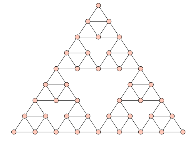
See also
There is another familly of graphs called Sierpinski graphs, where all vertices but 3 have valence 3. They are available using graphs.HanoiTowerGraph(3, n).
EXAMPLES:
sage: s4 = graphs.SierpinskiGasketGraph(4); s4
Graph on 42 vertices
sage: s4.size()
81
sage: s4.degree_histogram()
[0, 0, 3, 0, 39]
sage: s4.is_hamiltonian()
True
REFERENCES:
| [LLWC] | Chien-Hung Lin, Jia-Jie Liu, Yue-Li Wang, William Chung-Kung Yen, The Hub Number of Sierpinski-Like Graphs, Theory Comput Syst (2011), vol 49, doi:10.1007/s00224-010-9286-3 |
Returns the Sims-Gewirtz Graph.
This graph is obtained from the Higman Sims graph by considering the graph induced by the vertices at distance two from the vertices of an (any) edge. It is the only strongly regular graph with parameters \(v = 56, k = 10, \lambda = 0, \mu = 2\)
For more information on the Sylvester graph, see http://www.win.tue.nl/~aeb/graphs/Sims-Gewirtz.html or its Wikipedia page.
See also
EXAMPLE:
sage: g = graphs.SimsGewirtzGraph(); g
Sims-Gewirtz Graph: Graph on 56 vertices
sage: g.order()
56
sage: g.size()
280
sage: g.is_strongly_regular(parameters = True)
(56, 10, 0, 2)
Returns the Sousselier Graph.
The Sousselier graph is a hypohamiltonian graph on 16 vertices and 27 edges. For more information, see the corresponding Wikipedia page (in French).
EXAMPLES:
sage: g = graphs.SousselierGraph()
sage: g.order()
16
sage: g.size()
27
sage: g.radius()
2
sage: g.diameter()
3
sage: g.automorphism_group().cardinality()
2
sage: g.is_hamiltonian()
False
sage: g.delete_vertex(g.random_vertex())
sage: g.is_hamiltonian()
True
Returns a star graph with n+1 nodes.
A Star graph is a basic structure where one node is connected to all other nodes.
This constructor is dependent on NetworkX numeric labels.
PLOTTING: Upon construction, the position dictionary is filled to override the spring-layout algorithm. By convention, each star graph will be displayed with the first (0) node in the center, the second node (1) at the top, with the rest following in a counterclockwise manner. (0) is the node connected to all other nodes.
The star graph is a good opportunity to compare efficiency of filling a position dictionary vs. using the spring-layout algorithm for plotting. As far as display, the spring-layout should push all other nodes away from the (0) node, and thus look very similar to this constructor’s positioning.
EXAMPLES:
sage: import networkx
Compare the plots:
sage: n = networkx.star_graph(23)
sage: spring23 = Graph(n)
sage: posdict23 = graphs.StarGraph(23)
sage: spring23.show() # long time
sage: posdict23.show() # long time
View many star graphs as a Sage Graphics Array
With this constructor (i.e., the position dictionary filled)
sage: g = []
sage: j = []
sage: for i in range(9):
....: k = graphs.StarGraph(i+3)
....: g.append(k)
sage: for i in range(3):
....: n = []
....: for m in range(3):
....: n.append(g[3*i + m].plot(vertex_size=50, vertex_labels=False))
....: j.append(n)
sage: G = sage.plot.graphics.GraphicsArray(j)
sage: G.show() # long time
Compared to plotting with the spring-layout algorithm
sage: g = []
sage: j = []
sage: for i in range(9):
....: spr = networkx.star_graph(i+3)
....: k = Graph(spr)
....: g.append(k)
sage: for i in range(3):
....: n = []
....: for m in range(3):
....: n.append(g[3*i + m].plot(vertex_size=50, vertex_labels=False))
....: j.append(n)
sage: G = sage.plot.graphics.GraphicsArray(j)
sage: G.show() # long time
Returns the Sylvester Graph.
This graph is obtained from the Hoffman Singleton graph by considering the graph induced by the vertices at distance two from the vertices of an (any) edge.
For more information on the Sylvester graph, see http://www.win.tue.nl/~aeb/graphs/Sylvester.html.
See also
EXAMPLE:
sage: g = graphs.SylvesterGraph(); g
Sylvester Graph: Graph on 36 vertices
sage: g.order()
36
sage: g.size()
90
sage: g.is_regular(k=5)
True
Returns the Symplectic graph \(Sp(d,q)\)
The Symplectic Graph \(Sp(d,q)\) is built from a projective space of dimension \(d-1\) over a field \(F_q\), and a symplectic form \(f\). Two vertices \(u,v\) are made adjacent if \(f(u,v)=0\).
See the page on symplectic graphs on Andries Brouwer’s website.
INPUT:
EXAMPLES:
sage: g = graphs.SymplecticGraph(6,2)
sage: g.is_strongly_regular(parameters=True)
(63, 30, 13, 15)
sage: set(g.spectrum()) == {-5, 3, 30}
True
Returns the Szekeres Snark Graph.
The Szekeres graph is a snark with 50 vertices and 75 edges. For more information on this graph, see the Wikipedia article Szekeres_snark.
EXAMPLES:
sage: g = graphs.SzekeresSnarkGraph()
sage: g.order()
50
sage: g.size()
75
sage: g.chromatic_number()
3
Returns a tetrahedral graph (with 4 nodes).
A tetrahedron is a 4-sided triangular pyramid. The tetrahedral graph corresponds to the connectivity of the vertices of the tetrahedron. This graph is equivalent to a wheel graph with 4 nodes and also a complete graph on four nodes. (See examples below).
PLOTTING: The tetrahedral graph should be viewed in 3 dimensions. We chose to use the default spring-layout algorithm here, so that multiple iterations might yield a different point of reference for the user. We hope to add rotatable, 3-dimensional viewing in the future. In such a case, a string argument will be added to select the flat spring-layout over a future implementation.
EXAMPLES: Construct and show a Tetrahedral graph
sage: g = graphs.TetrahedralGraph()
sage: g.show() # long time
The following example requires networkx:
sage: import networkx as NX
Compare this Tetrahedral, Wheel(4), Complete(4), and the Tetrahedral plotted with the spring-layout algorithm below in a Sage graphics array:
sage: tetra_pos = graphs.TetrahedralGraph()
sage: tetra_spring = Graph(NX.tetrahedral_graph())
sage: wheel = graphs.WheelGraph(4)
sage: complete = graphs.CompleteGraph(4)
sage: g = [tetra_pos, tetra_spring, wheel, complete]
sage: j = []
sage: for i in range(2):
....: n = []
....: for m in range(2):
....: n.append(g[i + m].plot(vertex_size=50, vertex_labels=False))
....: j.append(n)
sage: G = sage.plot.graphics.GraphicsArray(j)
sage: G.show() # long time
Returns the Thomsen Graph.
The Thomsen Graph is actually a complete bipartite graph with \((n1, n2) = (3, 3)\). It is also called the Utility graph.
PLOTTING: See CompleteBipartiteGraph.
EXAMPLES:
sage: T = graphs.ThomsenGraph()
sage: T
Thomsen graph: Graph on 6 vertices
sage: T.graph6_string()
'EFz_'
sage: (graphs.ThomsenGraph()).show() # long time
Returns the Tietze Graph.
For more information on the Tietze Graph, see the Wikipedia article Tietze’s_graph.
EXAMPLES:
sage: g = graphs.TietzeGraph()
sage: g.order()
12
sage: g.size()
18
sage: g.diameter()
3
sage: g.girth()
3
sage: g.automorphism_group().cardinality()
12
sage: g.automorphism_group().is_isomorphic(groups.permutation.Dihedral(6))
True
Returns the graph generated by the tolerance representation tolrep.
The tolerance representation tolrep is described by the list \(((l_0,r_0,t_0), (l_1,r_1,t_1), ..., (l_k,r_k,t_k))\) where \(I_i = (l_i,r_i)\) denotes a closed interval on the real line with \(l_i < r_i\) and \(t_i\) a positive value, called tolerance. This representation generates the tolerance graph with the vertex set {0,1, ..., k} and the edge set \({(i,j): |I_i \cap I_j| \ge \min{t_i, t_j}}\) where \(|I_i \cap I_j|\) denotes the length of the intersection of \(I_i\) and \(I_j\).
INPUT:
Note
The vertices are named 0, 1, ..., k. The tolerance representation used to create the graph is saved with the graph and can be recovered using get_vertex() or get_vertices().
EXAMPLE:
The following code creates a tolerance representation tolrep, generates its tolerance graph g, and applies some checks:
sage: tolrep = [(1,4,3),(1,2,1),(2,3,1),(0,3,3)]
sage: g = graphs.ToleranceGraph(tolrep)
sage: g.get_vertex(3)
(0, 3, 3)
sage: neigh = g.neighbors(3)
sage: for v in neigh: print g.get_vertex(v)
(1, 2, 1)
(2, 3, 1)
sage: g.is_interval()
False
sage: g.is_weakly_chordal()
True
The intervals in the list need not be distinct
sage: tolrep2 = [(0,4,5),(1,2,1),(2,3,1),(0,4,5)]
sage: g2 = graphs.ToleranceGraph(tolrep2)
sage: g2.get_vertices()
{0: (0, 4, 5), 1: (1, 2, 1), 2: (2, 3, 1), 3: (0, 4, 5)}
sage: g2.is_isomorphic(g)
True
Real values are also allowed
sage: tolrep = [(0.1,3.3,4.4),(1.1,2.5,1.1),(1.4,4.4,3.3)]
sage: g = graphs.ToleranceGraph(tolrep)
sage: g.is_isomorphic(graphs.PathGraph(3))
True
TEST:
Giving negative third value:
sage: tolrep = [(0.1,3.3,-4.4),(1.1,2.5,1.1),(1.4,4.4,3.3)]
sage: g = graphs.ToleranceGraph(tolrep)
Traceback (most recent call last):
...
ValueError: Invalid tolerance representation at position 0; third value must be positive!
Returns a toroidal 6-regular grid.
The toroidal 6-regular grid is a 6-regular graph on \(n_1\times n_2\) vertices and its elements have coordinates \((i,j)\) for \(i \in \{0...i-1\}\) and \(j \in \{0...j-1\}\).
Its edges are those of the ToroidalGrid2dGraph(), to which are added the edges between \((i,j)\) and \(((i+1)\%n_1, (j+1)\%n_2)\).
INPUT:
EXAMPLE:
The toroidal 6-regular grid on \(25\) elements:
sage: g = graphs.Toroidal6RegularGrid2dGraph(5,5)
sage: g.is_regular(k=6)
True
sage: g.is_vertex_transitive()
True
sage: g.line_graph().is_vertex_transitive()
True
sage: g.automorphism_group().cardinality()
300
sage: g.is_hamiltonian()
True
TESTS:
Senseless input:
sage: graphs.Toroidal6RegularGrid2dGraph(5,2)
Traceback (most recent call last):
...
ValueError: Parameters n1 and n2 must be integers larger than 3 !
sage: graphs.Toroidal6RegularGrid2dGraph(2,0)
Traceback (most recent call last):
...
ValueError: Parameters n1 and n2 must be integers larger than 3 !
Returns a toroidal 2-dimensional grid graph with \(n_1n_2\) nodes (\(n_1\) rows and \(n_2\) columns).
The toroidal 2-dimensional grid with parameters \(n_1,n_2\) is the 2-dimensional grid graph with identical parameters to which are added the edges \(((i,0),(i,n_2-1))\) and \(((0,i),(n_1-1,i))\).
EXAMPLE:
The toroidal 2-dimensional grid is a regular graph, while the usual 2-dimensional grid is not
sage: tgrid = graphs.ToroidalGrid2dGraph(8,9)
sage: print tgrid
Toroidal 2D Grid Graph with parameters 8,9
sage: grid = graphs.Grid2dGraph(8,9)
sage: grid.is_regular()
False
sage: tgrid.is_regular()
True
Returns Tutte’s 12-Cage.
See the Wikipedia page on the Tutte 12-Cage.
EXAMPLES:
sage: g = graphs.Tutte12Cage()
sage: g.order()
126
sage: g.size()
189
sage: g.girth()
12
sage: g.diameter()
6
sage: g.show()
Returns the Tutte-Coxeter graph.
See the Wikipedia page on the Tutte-Coxeter Graph.
INPUT:
EXAMPLES:
sage: g = graphs.TutteCoxeterGraph()
sage: g.order()
30
sage: g.size()
45
sage: g.girth()
8
sage: g.diameter()
4
sage: g.show()
sage: graphs.TutteCoxeterGraph(embedding=1).show()
TESTS:
sage: graphs.TutteCoxeterGraph(embedding=3)
Traceback (most recent call last):
...
ValueError: The value of embedding must be 1 or 2.
Returns the Tutte Graph.
The Tutte graph is a 3-regular, 3-connected, and planar non-hamiltonian graph. For more information on the Tutte Graph, see the Wikipedia article Tutte_graph.
EXAMPLES:
sage: g = graphs.TutteGraph()
sage: g.order()
46
sage: g.size()
69
sage: g.is_planar()
True
sage: g.vertex_connectivity() # long
3
sage: g.girth()
4
sage: g.automorphism_group().cardinality()
3
sage: g.is_hamiltonian()
False
Returns the Wagner Graph.
See the Wikipedia page on the Wagner Graph.
EXAMPLES:
sage: g = graphs.WagnerGraph()
sage: g.order()
8
sage: g.size()
12
sage: g.girth()
4
sage: g.diameter()
2
sage: g.show()
Returns the Watkins Snark Graph.
The Watkins Graph is a snark with 50 vertices and 75 edges. For more information, see the Wikipedia article Watkins_snark.
EXAMPLES:
sage: g = graphs.WatkinsSnarkGraph()
sage: g.order()
50
sage: g.size()
75
sage: g.chromatic_number()
3
Returns the Wells graph.
For more information on the Wells graph (also called Armanios-Wells graph), see this page.
The implementation follows the construction given on page 266 of [BCN89]. This requires to create intermediate graphs and run a small isomorphism test, while everything could be replaced by a pre-computed list of edges : I believe that it is better to keep “the recipe” in the code, however, as it is quite unlikely that this could become the most time-consuming operation in any sensible algorithm, and .... “preserves knowledge”, which is what open-source software is meant to do.
EXAMPLES:
sage: g = graphs.WellsGraph(); g
Wells graph: Graph on 32 vertices
sage: g.order()
32
sage: g.size()
80
sage: g.girth()
5
sage: g.diameter()
4
sage: g.chromatic_number()
4
sage: g.is_regular(k=5)
True
REFERENCES:
| [BCN89] | A. E. Brouwer, A. M. Cohen, A. Neumaier, Distance-Regular Graphs, Springer, 1989. |
Returns a Wheel graph with n nodes.
A Wheel graph is a basic structure where one node is connected to all other nodes and those (outer) nodes are connected cyclically.
This constructor depends on NetworkX numeric labels.
PLOTTING: Upon construction, the position dictionary is filled to override the spring-layout algorithm. By convention, each wheel graph will be displayed with the first (0) node in the center, the second node at the top, and the rest following in a counterclockwise manner.
With the wheel graph, we see that it doesn’t take a very large n at all for the spring-layout to give a counter-intuitive display. (See Graphics Array examples below).
EXAMPLES: We view many wheel graphs with a Sage Graphics Array, first with this constructor (i.e., the position dictionary filled):
sage: g = []
sage: j = []
sage: for i in range(9):
... k = graphs.WheelGraph(i+3)
... g.append(k)
...
sage: for i in range(3):
... n = []
... for m in range(3):
... n.append(g[3*i + m].plot(vertex_size=50, vertex_labels=False))
... j.append(n)
...
sage: G = sage.plot.graphics.GraphicsArray(j)
sage: G.show() # long time
Next, using the spring-layout algorithm:
sage: import networkx
sage: g = []
sage: j = []
sage: for i in range(9):
... spr = networkx.wheel_graph(i+3)
... k = Graph(spr)
... g.append(k)
...
sage: for i in range(3):
... n = []
... for m in range(3):
... n.append(g[3*i + m].plot(vertex_size=50, vertex_labels=False))
... j.append(n)
...
sage: G = sage.plot.graphics.GraphicsArray(j)
sage: G.show() # long time
Compare the plotting:
sage: n = networkx.wheel_graph(23)
sage: spring23 = Graph(n)
sage: posdict23 = graphs.WheelGraph(23)
sage: spring23.show() # long time
sage: posdict23.show() # long time
Returns the Wiener-Araya Graph.
The Wiener-Araya Graph is a planar hypohamiltonian graph on 42 vertices and 67 edges. For more information, see the Wolfram Page on the Wiener-Araya Graph or its (french) Wikipedia page.
EXAMPLES:
sage: g = graphs.WienerArayaGraph()
sage: g.order()
42
sage: g.size()
67
sage: g.girth()
4
sage: g.is_planar()
True
sage: g.is_hamiltonian() # not tested -- around 30s long
False
sage: g.delete_vertex(g.random_vertex())
sage: g.is_hamiltonian()
True
Returns the Graph of all the countries, in which two countries are adjacent in the graph if they have a common boundary.
This graph has been built from the data available in The CIA World Factbook [CIA] (2009-08-21).
The returned graph G has a member G.gps_coordinates equal to a dictionary containing the GPS coordinates of each country’s capital city.
EXAMPLE:
sage: g=graphs.WorldMap()
sage: g.has_edge("France","Italy")
True
sage: g.gps_coordinates["Bolivia"]
[[17, 'S'], [65, 'W']]
sage: sorted(g.connected_component_containing_vertex('Ireland'))
['Ireland', 'United Kingdom']
REFERENCE:
| [CIA] | CIA Factbook 09 https://www.cia.gov/library/publications/the-world-factbook/ |
Return the three Chang graphs.
Three of the four strongly regular graphs of parameters \((28,12,6,4)\) are called the Chang graphs. The fourth is the line graph of \(K_8\). For more information about the Chang graphs, see Wikipedia article Chang_graphs or http://www.win.tue.nl/~aeb/graphs/Chang.html.
EXAMPLES:
sage: chang_graphs = graphs.chang_graphs()
sage: four_srg = chang_graphs + [graphs.CompleteGraph(8).line_graph()]
sage: for g in four_srg:
....: print g.is_strongly_regular(parameters=True)
(28, 12, 6, 4)
(28, 12, 6, 4)
(28, 12, 6, 4)
(28, 12, 6, 4)
sage: from itertools import combinations
sage: for g1,g2 in combinations(four_srg,2):
....: assert not g1.is_isomorphic(g2)
Find all sets of graphs on vertices vertices (with possible restrictions) which are cospectral with respect to a constructed matrix.
INPUT:
vertices - The number of vertices in the graphs to be tested
matrix_function - A function taking a graph and giving back a matrix. This defaults to the adjacency matrix. The spectra examined are the spectra of these matrices.
graphs - One of three things:
- None (default) - test all graphs having vertices vertices
- a function taking a graph and returning True or False - test only the graphs on vertices vertices for which the function returns True
- a list of graphs (or other iterable object) - these graphs are tested for cospectral sets. In this case, vertices is ignored.
OUTPUT:
A list of lists of graphs. Each sublist will be a list of cospectral graphs (lists of cadinality 1 being omitted).
See also
Graph.is_strongly_regular() – tests whether a graph is strongly regular and/or returns its parameters.
EXAMPLES:
sage: g=graphs.cospectral_graphs(5)
sage: sorted(sorted(g.graph6_string() for g in glist) for glist in g)
[['Dr?', 'Ds_']]
sage: g[0][1].am().charpoly()==g[0][1].am().charpoly()
True
There are two sets of cospectral graphs on six vertices with no isolated vertices:
sage: g=graphs.cospectral_graphs(6, graphs=lambda x: min(x.degree())>0)
sage: sorted(sorted(g.graph6_string() for g in glist) for glist in g)
[['Ep__', 'Er?G'], ['ExGg', 'ExoG']]
sage: g[0][1].am().charpoly()==g[0][1].am().charpoly()
True
sage: g[1][1].am().charpoly()==g[1][1].am().charpoly()
True
There is one pair of cospectral trees on eight vertices:
sage: g=graphs.cospectral_graphs(6, graphs=graphs.trees(8))
sage: sorted(sorted(g.graph6_string() for g in glist) for glist in g)
[['GiPC?C', 'GiQCC?']]
sage: g[0][1].am().charpoly()==g[0][1].am().charpoly()
True
There are two sets of cospectral graphs (with respect to the Laplacian matrix) on six vertices:
sage: g=graphs.cospectral_graphs(6, matrix_function=lambda g: g.laplacian_matrix())
sage: sorted(sorted(g.graph6_string() for g in glist) for glist in g)
[['Edq_', 'ErcG'], ['Exoo', 'EzcG']]
sage: g[0][1].laplacian_matrix().charpoly()==g[0][1].laplacian_matrix().charpoly()
True
sage: g[1][1].laplacian_matrix().charpoly()==g[1][1].laplacian_matrix().charpoly()
True
To find cospectral graphs with respect to the normalized Laplacian, assuming the graphs do not have an isolated vertex, it is enough to check the spectrum of the matrix \(D^{-1}A\), where \(D\) is the diagonal matrix of vertex degrees, and A is the adjacency matrix. We find two such cospectral graphs (for the normalized Laplacian) on five vertices:
sage: def DinverseA(g):
... A=g.adjacency_matrix().change_ring(QQ)
... for i in range(g.order()):
... A.rescale_row(i, 1/len(A.nonzero_positions_in_row(i)))
... return A
sage: g=graphs.cospectral_graphs(5, matrix_function=DinverseA, graphs=lambda g: min(g.degree())>0)
sage: sorted(sorted(g.graph6_string() for g in glist) for glist in g)
[['Dlg', 'Ds_']]
sage: g[0][1].laplacian_matrix(normalized=True).charpoly()==g[0][1].laplacian_matrix(normalized=True).charpoly()
True
Returns a generator which creates fullerene graphs using the buckygen generator (see [buckygen]).
INPUT:
OUTPUT:
A generator which will produce the fullerene graphs as Sage graphs with an embedding set. These will be simple graphs: no loops, no multiple edges, no directed edges.
See also
EXAMPLES:
There are 1812 isomers of \(\textrm{C}_{60}\), i.e., 1812 fullerene graphs on 60 vertices:
sage: gen = graphs.fullerenes(60) # optional buckygen
sage: len(list(gen)) # optional buckygen
1812
However, there is only one IPR fullerene graph on 60 vertices: the famous Buckminster Fullerene:
sage: gen = graphs.fullerenes(60, ipr=True) # optional buckygen
sage: next(gen) # optional buckygen
Graph on 60 vertices
sage: next(gen) # optional buckygen
Traceback (most recent call last):
...
StopIteration
The unique fullerene graph on 20 vertices is isomorphic to the dodecahedron graph.
sage: gen = graphs.fullerenes(20) # optional buckygen
sage: g = next(gen) # optional buckygen
sage: g.is_isomorphic(graphs.DodecahedralGraph()) # optional buckygen
True
sage: g.get_embedding() # optional buckygen
{1: [2, 3, 4],
2: [1, 5, 6],
3: [1, 7, 8],
4: [1, 9, 10],
5: [2, 10, 11],
6: [2, 12, 7],
7: [3, 6, 13],
8: [3, 14, 9],
9: [4, 8, 15],
10: [4, 16, 5],
11: [5, 17, 12],
12: [6, 11, 18],
13: [7, 18, 14],
14: [8, 13, 19],
15: [9, 19, 16],
16: [10, 15, 17],
17: [11, 16, 20],
18: [12, 20, 13],
19: [14, 20, 15],
20: [17, 19, 18]}
sage: g.plot3d(layout='spring') # optional buckygen
Graphics3d Object
REFERENCE:
| [buckygen] | G. Brinkmann, J. Goedgebeur and B.D. McKay, Generation of Fullerenes, Journal of Chemical Information and Modeling, 52(11):2910-2918, 2012. |
Returns a generator which creates fusenes and benzenoids using the benzene generator (see [benzene]). Fusenes are planar polycyclic hydrocarbons with all bounded faces hexagons. Benzenoids are fusenes that are subgraphs of the hexagonal lattice.
INPUT:
OUTPUT:
A generator which will produce the fusenes as Sage graphs with an embedding set. These will be simple graphs: no loops, no multiple edges, no directed edges.
See also
EXAMPLES:
There is a unique fusene with 2 hexagons:
sage: gen = graphs.fusenes(2) # optional benzene
sage: len(list(gen)) # optional benzene
1
This fusene is naphtalene (\(\textrm{C}_{10}\textrm{H}_{8}\)). In the fusene graph the H-atoms are not stored, so this is a graph on just 10 vertices:
sage: gen = graphs.fusenes(2) # optional benzene
sage: next(gen) # optional benzene
Graph on 10 vertices
sage: next(gen) # optional benzene
Traceback (most recent call last):
...
StopIteration
There are 6505 benzenoids with 9 hexagons:
sage: gen = graphs.fusenes(9, benzenoids=True) # optional benzene
sage: len(list(gen)) # optional benzene
6505
REFERENCE:
| [benzene] | G. Brinkmann, G. Caporossi and P. Hansen, A Constructive Enumeration of Fusenes and Benzenoids, Journal of Algorithms, 45:155-166, 2002. |
Returns the 9 forbidden subgraphs of a line graph.
Wikipedia article on the line graphs
The graphs are returned in the ordering given by the Wikipedia drawing, read from left to right and from top to bottom.
EXAMPLE:
sage: graphs.line_graph_forbidden_subgraphs()
[Claw graph: Graph on 4 vertices,
Graph on 6 vertices,
Graph on 6 vertices,
Graph on 5 vertices,
Graph on 6 vertices,
Graph on 6 vertices,
Graph on 6 vertices,
Graph on 6 vertices,
Graph on 5 vertices]
Returns a generator which creates graphs from nauty’s geng program.
Note
Due to license restrictions, the nauty package is distributed as a Sage optional package. At a system command line, execute sage -i nauty to see the nauty license and install the package.
INPUT:
The possible options, obtained as output of geng --help:
n : the number of vertices
mine:maxe : a range for the number of edges
#:0 means '# or more' except in the case 0:0
res/mod : only generate subset res out of subsets 0..mod-1
-c : only write connected graphs
-C : only write biconnected graphs
-t : only generate triangle-free graphs
-f : only generate 4-cycle-free graphs
-b : only generate bipartite graphs
(-t, -f and -b can be used in any combination)
-m : save memory at the expense of time (only makes a
difference in the absence of -b, -t, -f and n <= 28).
-d# : a lower bound for the minimum degree
-D# : a upper bound for the maximum degree
-v : display counts by number of edges
-l : canonically label output graphs
-q : suppress auxiliary output (except from -v)
Options which cause geng to use an output format different than the graph6 format are not listed above (-u, -g, -s, -y, -h) as they will confuse the creation of a Sage graph. The res/mod option can be useful when using the output in a routine run several times in parallel.
OUTPUT:
A generator which will produce the graphs as Sage graphs. These will be simple graphs: no loops, no multiple edges, no directed edges.
See also
Graph.is_strongly_regular() – tests whether a graph is strongly regular and/or returns its parameters.
EXAMPLES:
The generator can be used to construct graphs for testing, one at a time (usually inside a loop). Or it can be used to create an entire list all at once if there is sufficient memory to contain it.
sage: gen = graphs.nauty_geng("2") # optional nauty
sage: next(gen) # optional nauty
Graph on 2 vertices
sage: next(gen) # optional nauty
Graph on 2 vertices
sage: next(gen) # optional nauty
Traceback (most recent call last):
...
StopIteration: Exhausted list of graphs from nauty geng
A list of all graphs on 7 vertices. This agrees with OEIS sequence A000088.
sage: gen = graphs.nauty_geng("7") # optional nauty
sage: len(list(gen)) # optional nauty
1044
A list of just the connected graphs on 7 vertices. This agrees with OEIS sequence A001349.
sage: gen = graphs.nauty_geng("7 -c") # optional nauty
sage: len(list(gen)) # optional nauty
853
The debug switch can be used to examine geng’s reaction to the input in the options string. We illustrate success. (A failure will be a string beginning with “>E”.) Passing the “-q” switch to geng will supress the indicator of a successful initiation.
sage: gen = graphs.nauty_geng("4", debug=True) # optional nauty
sage: print next(gen) # optional nauty
>A geng -d0D3 n=4 e=0-6
Returns the Petersen family
The Petersen family is a collection of 7 graphs which are the forbidden minors of the linklessly embeddable graphs. For more information see the Wikipedia article Petersen_family.
INPUT:
EXAMPLE:
sage: graphs.petersen_family()
[Petersen graph: Graph on 10 vertices,
Complete graph: Graph on 6 vertices,
Multipartite Graph with set sizes [3, 3, 1]: Graph on 7 vertices,
Graph on 8 vertices,
Graph on 9 vertices,
Graph on 7 vertices,
Graph on 8 vertices]
The two different inputs generate the same graphs:
sage: F1 = graphs.petersen_family(generate=False)
sage: F2 = graphs.petersen_family(generate=True)
sage: F1 = [g.canonical_label().graph6_string() for g in F1]
sage: F2 = [g.canonical_label().graph6_string() for g in F2]
sage: set(F1) == set(F2)
True
An iterator over connected planar graphs using the plantri generator.
This uses the plantri generator (see [plantri]) which is available through the optional package plantri.
Note
The non-3-connected graphs will be returned several times, with all its possible embeddings.
INPUT:
OUTPUT:
An iterator which will produce all planar graphs with the given number of vertices as Sage graphs with an embedding set. These will be simple graphs (no loops, no multiple edges, no directed edges) unless the option dual=True is used.
See also
EXAMPLES:
There are 6 planar graphs on 4 vertices:
sage: gen = graphs.planar_graphs(4) # optional plantri
sage: len(list(gen)) # optional plantri
6
Three of these planar graphs are bipartite:
sage: gen = graphs.planar_graphs(4, only_bipartite=True) # optional plantri
sage: len(list(gen)) # optional plantri
3
Setting dual=True gives the planar dual graphs:
sage: gen = graphs.planar_graphs(4, dual=True) # optional plantri
sage: [u for u in list(gen)] # optional plantri
[Graph on 4 vertices,
Multi-graph on 3 vertices,
Multi-graph on 2 vertices,
Looped multi-graph on 2 vertices,
Looped multi-graph on 1 vertex,
Looped multi-graph on 1 vertex]
The cycle of length 4 is the only 2-connected bipartite planar graph on 4 vertices:
sage: l = list(graphs.planar_graphs(4, minimum_connectivity=2, only_bipartite=True)) # optional plantri
sage: l[0].get_embedding() # optional plantri
{1: [2, 3],
2: [1, 4],
3: [1, 4],
4: [2, 3]}
There is one planar graph with one vertex. This graph obviously has minimum degree equal to 0:
sage: list(graphs.planar_graphs(1)) # optional plantri
[Graph on 1 vertex]
sage: list(graphs.planar_graphs(1, minimum_degree=1)) # optional plantri
[]
TESTS:
The number of edges in a planar graph is equal to the number of edges in its dual:
sage: planar = list(graphs.planar_graphs(5,dual=True)) # optional -- plantri
sage: dual_planar = list(graphs.planar_graphs(5,dual=False)) # optional -- plantri
sage: planar_sizes = [g.size() for g in planar] # optional -- plantri
sage: dual_planar_sizes = [g.size() for g in dual_planar] # optional -- plantri
sage: planar_sizes == dual_planar_sizes # optional -- plantri
True
REFERENCE:
| [plantri] | (1, 2, 3) G. Brinkmann and B.D. McKay, Fast generation of planar graphs, MATCH-Communications in Mathematical and in Computer Chemistry, 58(2):323-357, 2007. |
An iterator over planar quadrangulations using the plantri generator.
This uses the plantri generator (see [plantri]) which is available through the optional package plantri.
INPUT:
OUTPUT:
An iterator which will produce all planar quadrangulations with the given number of vertices as Sage graphs with an embedding set. These will be simple graphs (no loops, no multiple edges, no directed edges).
See also
EXAMPLES:
The cube is the only 3-connected planar quadrangulation on 8 vertices:
sage: gen = graphs.quadrangulations(8, minimum_connectivity=3) # optional plantri
sage: g = next(gen) # optional plantri
sage: g.is_isomorphic(graphs.CubeGraph(3)) # optional plantri
True
sage: next(gen) # optional plantri
Traceback (most recent call last):
...
StopIteration
An overview of the number of quadrangulations on up to 12 vertices. This agrees with OEIS sequence A113201:
sage: for i in range(4,13): # optional plantri
....: L = len(list(graphs.quadrangulations(i))) # optional plantri
....: print("{:2d} {:3d}".format(i,L)) # optional plantri
4 1
5 1
6 2
7 3
8 9
9 18
10 62
11 198
12 803
There are 2 planar quadrangulation on 12 vertices that do not have a non-facial quadrangle:
sage: len([g for g in graphs.quadrangulations(12, no_nonfacial_quadrangles=True)]) # optional plantri
2
Setting dual=True gives the planar dual graphs:
sage: [len(g) for g in graphs.quadrangulations(12, no_nonfacial_quadrangles=True, dual=True)] # optional plantri
[10, 10]
Returns a generator of the distinct trees on a fixed number of vertices.
INPUT:
OUTPUT:
A generator which creates an exhaustive, duplicate-free listing of the connected free (unlabeled) trees with vertices number of vertices. A tree is a graph with no cycles.
ALGORITHM:
Uses an algorithm that generates each new tree in constant time. See the documentation for, and implementation of, the sage.graphs.trees module, including a citation.
EXAMPLES:
We create an iterator, then loop over its elements.
sage: tree_iterator = graphs.trees(7)
sage: for T in tree_iterator:
... print T.degree_sequence()
[2, 2, 2, 2, 2, 1, 1]
[3, 2, 2, 2, 1, 1, 1]
[3, 2, 2, 2, 1, 1, 1]
[4, 2, 2, 1, 1, 1, 1]
[3, 3, 2, 1, 1, 1, 1]
[3, 3, 2, 1, 1, 1, 1]
[4, 3, 1, 1, 1, 1, 1]
[3, 2, 2, 2, 1, 1, 1]
[4, 2, 2, 1, 1, 1, 1]
[5, 2, 1, 1, 1, 1, 1]
[6, 1, 1, 1, 1, 1, 1]
The number of trees on the first few vertex counts. This is sequence A000055 in Sloane’s OEIS.
sage: [len(list(graphs.trees(i))) for i in range(0, 15)]
[1, 1, 1, 1, 2, 3, 6, 11, 23, 47, 106, 235, 551, 1301, 3159]
An iterator over connected planar triangulations using the plantri generator.
This uses the plantri generator (see [plantri]) which is available through the optional package plantri.
INPUT:
OUTPUT:
An iterator which will produce all planar triangulations with the given number of vertices as Sage graphs with an embedding set. These will be simple graphs (no loops, no multiple edges, no directed edges).
See also
EXAMPLES:
The unique planar embedding of the \(K_4\) is the only planar triangulations on 4 vertices:
sage: gen = graphs.triangulations(4) # optional plantri
sage: [g.get_embedding() for g in gen] # optional plantri
[{1: [2, 3, 4], 2: [1, 4, 3], 3: [1, 2, 4], 4: [1, 3, 2]}]
but, of course, this graph is not eulerian:
sage: gen = graphs.triangulations(4, only_eulerian=True) # optional plantri
sage: len(list(gen)) # optional plantri
0
The unique eulerian triangulation on 6 vertices is isomorphic to the octahedral graph.
sage: gen = graphs.triangulations(6, only_eulerian=True) # optional plantri
sage: g = next(gen) # optional plantri
sage: g.is_isomorphic(graphs.OctahedralGraph()) # optional plantri
True
An overview of the number of 5-connected triangulations on up to 22 vertices. This agrees with OEIS sequence A081621:
sage: for i in range(12, 23): # optional plantri
....: L = len(list(graphs.triangulations(i, minimum_connectivity=5))) # optional plantri
....: print("{} {:3d}".format(i,L)) # optional plantri
12 1
13 0
14 1
15 1
16 3
17 4
18 12
19 23
20 71
21 187
22 627
The minimum connectivity can be at most the minimum degree:
sage: gen = next(graphs.triangulations(10, minimum_degree=3, minimum_connectivity=5)) # optional plantri
Traceback (most recent call last):
...
ValueError: Minimum connectivity can be at most the minimum degree.
There are 5 triangulations with 9 vertices and minimum degree equal to 4 that are 3-connected, but only one of them is not 4-connected:
sage: len([g for g in graphs.triangulations(9, minimum_degree=4, minimum_connectivity=3)]) # optional plantri
5
sage: len([g for g in graphs.triangulations(9, minimum_degree=4, minimum_connectivity=3, exact_connectivity=True)]) # optional plantri
1
Setting dual=True gives the planar dual graphs:
sage: [len(g) for g in graphs.triangulations(9, minimum_degree=4, minimum_connectivity=3, dual=True)] # optional plantri
[14, 14, 14, 14, 14]
TESTS:
sage: [g.size() for g in graphs.triangulations(6, minimum_connectivity=3)] # optional plantri
[12, 12]
Main function for exhaustive generation. Recursive traversal of a canonically generated tree of isomorph free graphs satisfying a given property.
INPUT:
EXAMPLES:
sage: from sage.graphs.graph_generators import canaug_traverse_edge
sage: G = Graph(3)
sage: list(canaug_traverse_edge(G, [], lambda x: True))
[Graph on 3 vertices, ... Graph on 3 vertices]
The best way to access this function is through the graphs() iterator:
Print graphs on 3 or less vertices.
sage: for G in graphs(3):
... print G
...
Graph on 3 vertices
Graph on 3 vertices
Graph on 3 vertices
Graph on 3 vertices
Print digraphs on 3 or less vertices.
sage: for G in digraphs(3):
... print G
...
Digraph on 3 vertices
Digraph on 3 vertices
...
Digraph on 3 vertices
Digraph on 3 vertices
Main function for exhaustive generation. Recursive traversal of a canonically generated tree of isomorph free (di)graphs satisfying a given property.
INPUT:
EXAMPLES:
sage: from sage.graphs.graph_generators import canaug_traverse_vert
sage: list(canaug_traverse_vert(Graph(), [], 3, lambda x: True))
[Graph on 0 vertices, ... Graph on 3 vertices]
The best way to access this function is through the graphs() iterator:
Print graphs on 3 or less vertices.
sage: for G in graphs(3, augment='vertices'):
... print G
...
Graph on 0 vertices
Graph on 1 vertex
Graph on 2 vertices
Graph on 3 vertices
Graph on 3 vertices
Graph on 3 vertices
Graph on 2 vertices
Graph on 3 vertices
Print digraphs on 2 or less vertices.
sage: for D in digraphs(2, augment='vertices'):
... print D
...
Digraph on 0 vertices
Digraph on 1 vertex
Digraph on 2 vertices
Digraph on 2 vertices
Digraph on 2 vertices
Helper function for exhaustive generation.
At the start, check_aut is given a set of generators for the automorphism group, aut_gens. We already know we are looking for an element of the auto- morphism group that sends cut_vert to n, and check_aut generates these for the canaug_traverse function.
EXAMPLE: Note that the last two entries indicate that none of the automorphism group has yet been searched - we are starting at the identity [0, 1, 2, 3] and so far that is all we have seen. We return automorphisms mapping 2 to 3.
sage: from sage.graphs.graph_generators import check_aut
sage: list( check_aut( [ [0, 3, 2, 1], [1, 0, 3, 2], [2, 1, 0, 3] ], 2, 3))
[[1, 0, 3, 2], [1, 2, 3, 0]]
Helper function for exhaustive generation.
At the start, check_aut_edge is given a set of generators for the automorphism group, aut_gens. We already know we are looking for an element of the auto- morphism group that sends cut_edge to {i, j}, and check_aut generates these for the canaug_traverse function.
EXAMPLE: Note that the last two entries indicate that none of the automorphism group has yet been searched - we are starting at the identity [0, 1, 2, 3] and so far that is all we have seen. We return automorphisms mapping 2 to 3.
sage: from sage.graphs.graph_generators import check_aut
sage: list( check_aut( [ [0, 3, 2, 1], [1, 0, 3, 2], [2, 1, 0, 3] ], 2, 3))
[[1, 0, 3, 2], [1, 2, 3, 0]]