basics.sagews

R Basics

Just a demo, how R can be called from Sage to do something useful.

Note: every block of code starts with %r to switch to R-mode. Use %default_mode r in a single bock to switch r to be the default.

%r
x <- c(1,4,3,4,3,2,3,2,3,6,3)
summary(x)

Min. 1st Qu. Median Mean 3rd Qu. Max. 1.000 2.500 3.000 3.091 3.500 6.000

%r
x[1]
x[2]

1

4

%r
z <- sample(-5:5, 30, replace=T)
z
summary(z)

1. 5
2. 2
3. 3
4. -1
5. -1
6. -1
7. 2
8. -5
9. -4
10. -5
11. 0
12. -5
13. -3
14. 2
15. 5
16. 1
17. 5
18. 5
19. 2
20. 3
21. 3
22. 3
23. 5
24. -2
25. -1
26. -1
27. -5
28. 2
29. 3
30. -5

Min. 1st Qu. Median Mean 3rd Qu. Max. -5.00 -1.75 1.50 0.40 3.00 5.00

%r
plot(-5:5, sample(-5:5, 11, replace=F))

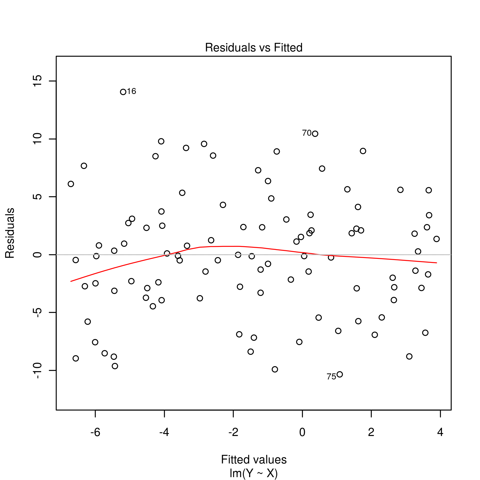
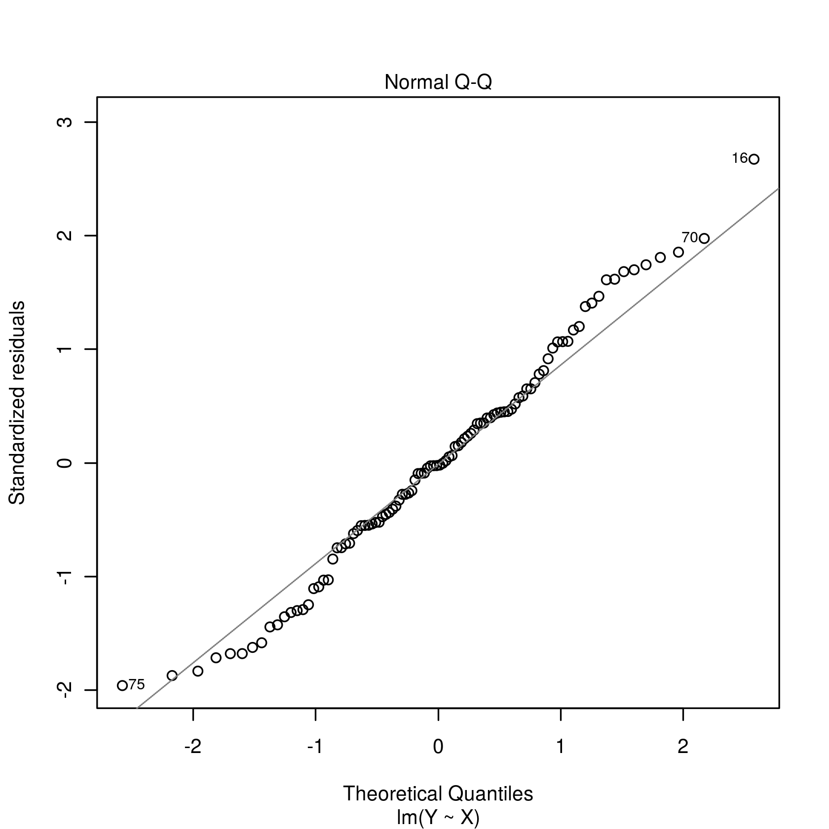
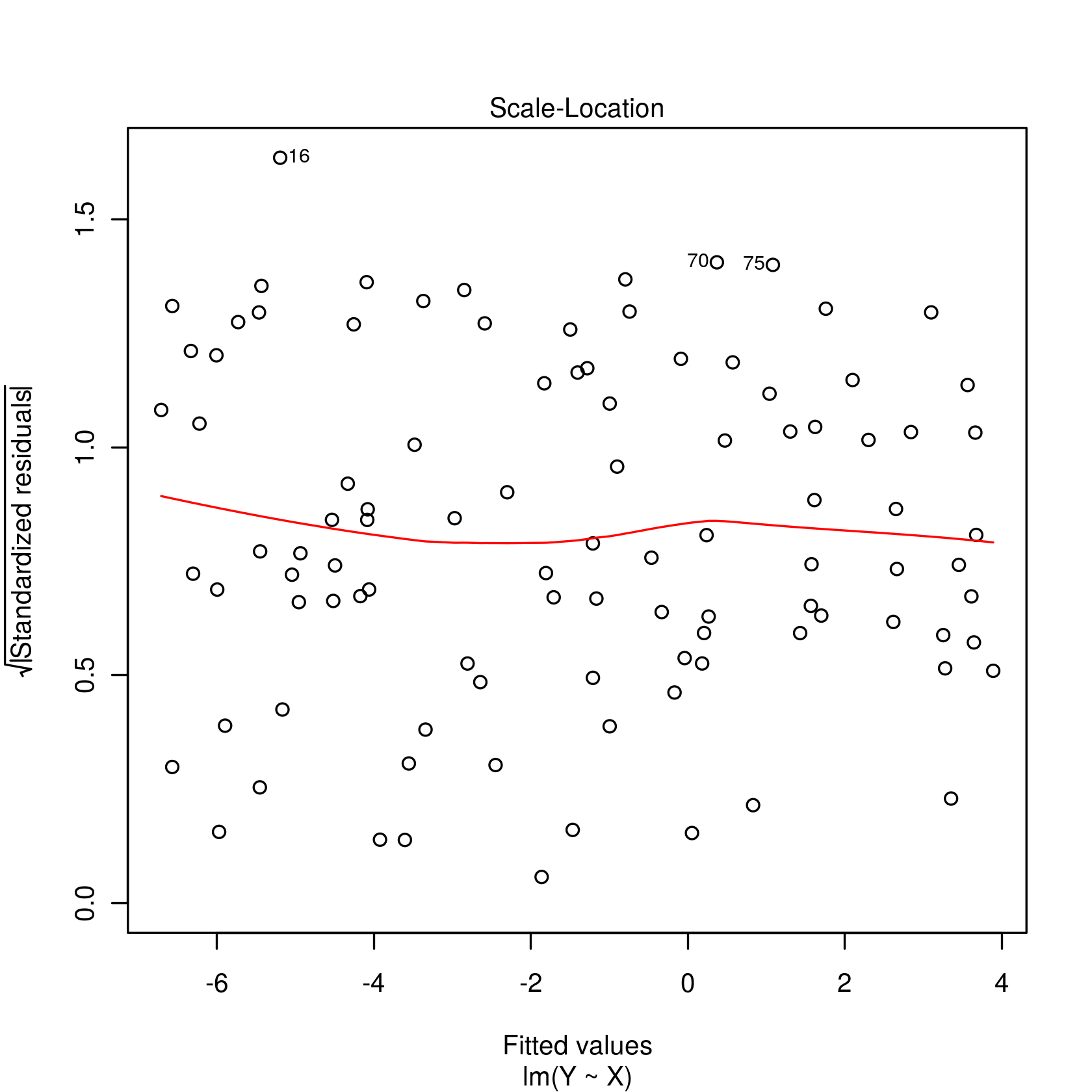
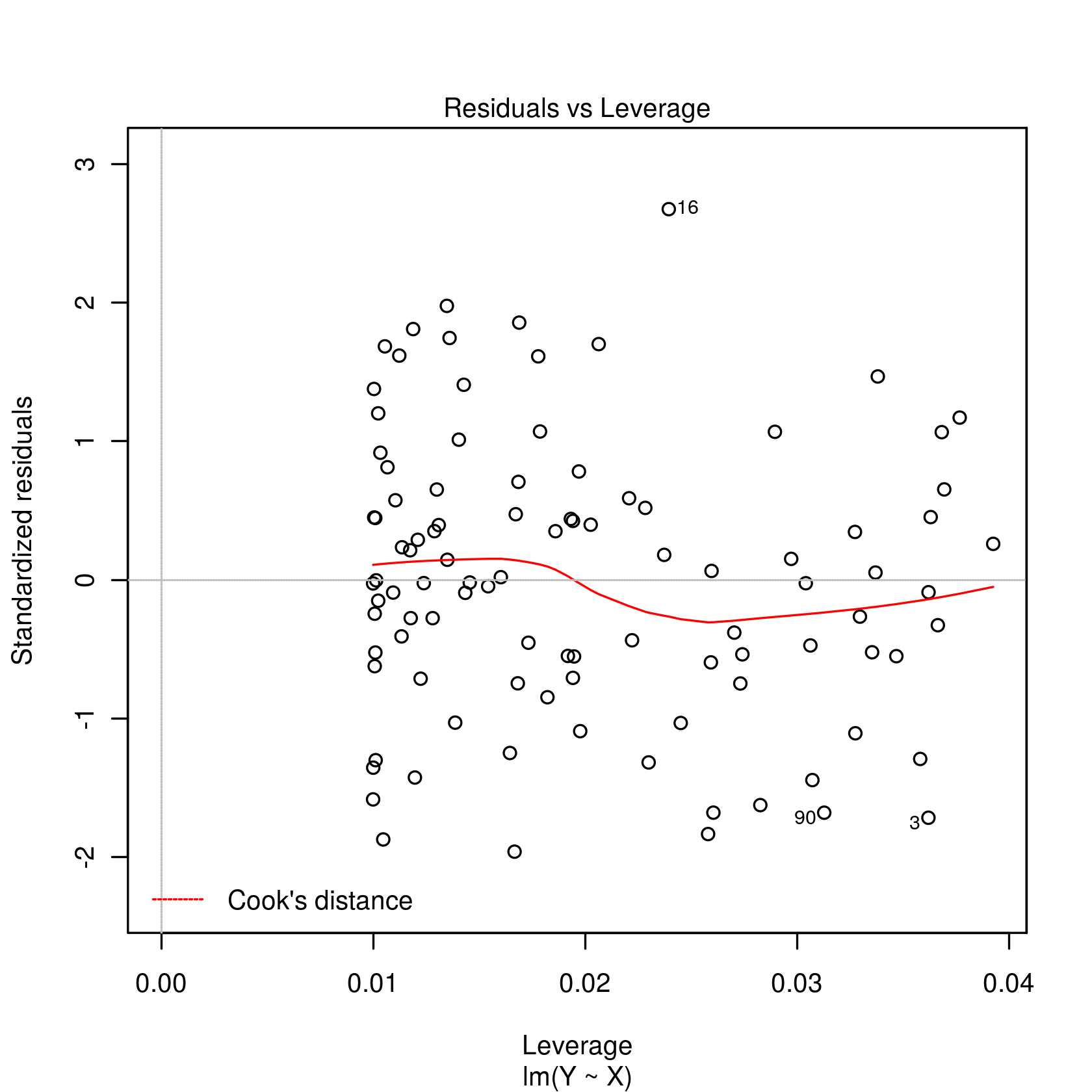
Linear Regression

%r
X <- sort(runif(100, -5,5))
Y <- -2 + 1.1 * X + rnorm(100, 0, 5)
lmobj <- lm(Y ~ X)
summary(lmobj)

Call: lm(formula = Y ~ X) Residuals: Min 1Q Median 3Q Max -10.3505 -3.1704 -0.1131 3.0550 14.0648 Coefficients: Estimate Std. Error t value Pr(>|t|) (Intercept) -1.3877 0.5326 -2.606 0.0106 * X 1.0741 0.1821 5.900 5.2e-08 *** --- Signif. codes: 0 ‘***’ 0.001 ‘**’ 0.01 ‘*’ 0.05 ‘.’ 0.1 ‘ ’ 1 Residual standard error: 5.323 on 98 degrees of freedom Multiple R-squared: 0.2621, Adjusted R-squared: 0.2546 F-statistic: 34.81 on 1 and 98 DF, p-value: 5.199e-08

It is also possible to plot the R-object lmobj to learn more about the linear regression.

%r
plot(lmobj)