CoCalc Logo Icon
StoreFeaturesDocsShareSupportNewsAboutSign UpSign In
DanielBarnes18

Real-time collaboration for Jupyter Notebooks, Linux Terminals, LaTeX, VS Code, R IDE, and more,
all in one place. Commercial Alternative to JupyterHub.

GitHub Repository: DanielBarnes18/IBM-Data-Science-Professional-Certificate
Path: blob/main/08. Data Visualization with Python/01. Preparing the Canada Immigration Dataset.ipynb
Views: 4585
Kernel: Python 3.7.6 ('base')

Preparing the Canada Immigration Dataset with pandas

Toolkits: The course heavily relies on pandas and Numpy for data wrangling, analysis, and visualization. The primary plotting library we will explore in the course is Matplotlib.

Dataset: Immigration to Canada from 1980 to 2013 - International migration flows to and from selected countries - The 2015 revision from United Nation's website.

The dataset contains annual data on the flows of international migrants as recorded by the countries of destination. The data presents both inflows and outflows according to the place of birth, citizenship or place of previous / next residence both for foreigners and nationals. In this lab, we will focus on the Canadian Immigration data.
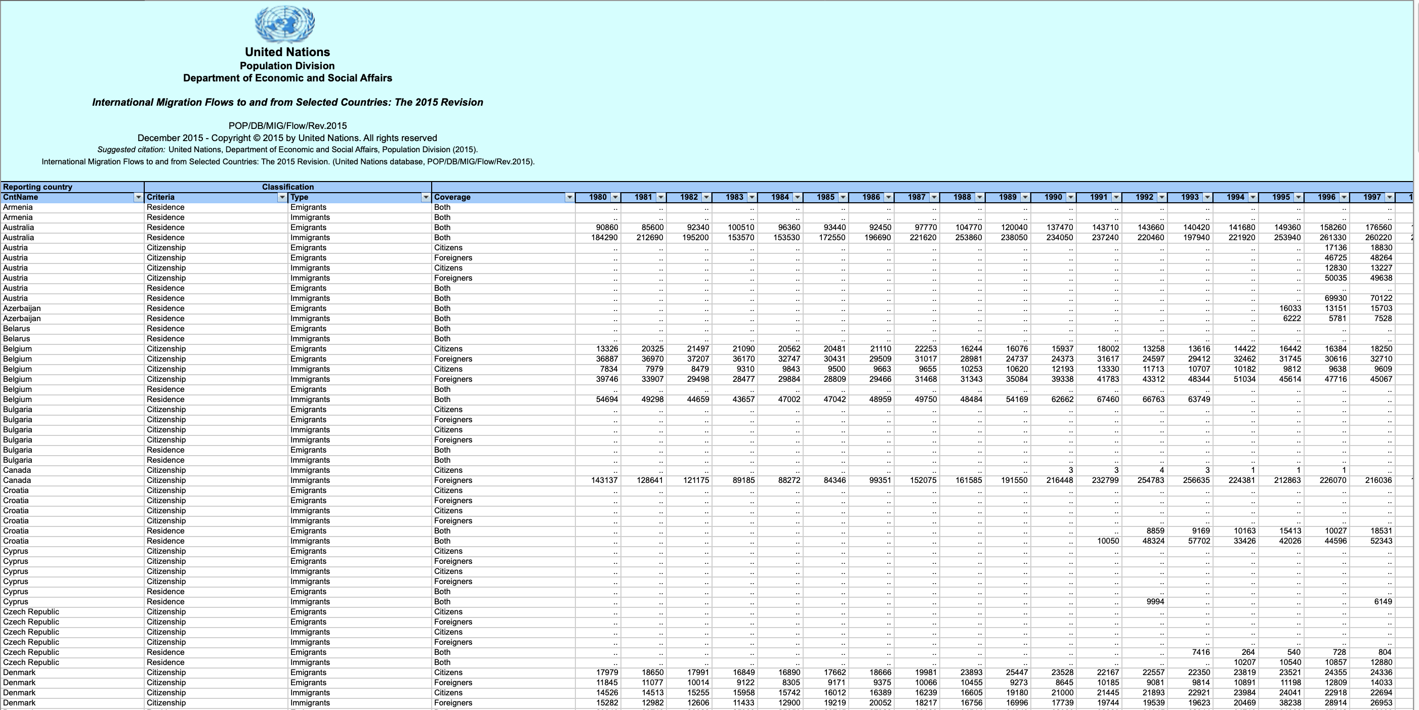
Data Preview

The Canada Immigration dataset can be fetched from here.


Downloading and Prepping Data

#Imports import numpy as np import pandas as pd
#install the openpyxl package #!python -m pip install openpyxl

Download the dataset and read it into a pandas dataframe.

df_can = pd.read_excel( 'https://cf-courses-data.s3.us.cloud-object-storage.appdomain.cloud/IBMDeveloperSkillsNetwork-DV0101EN-SkillsNetwork/Data%20Files/Canada.xlsx', sheet_name='Canada by Citizenship', skiprows=range(20), skipfooter=2 )

Explore the dataset

#First 5 items in the dataset df_can.head()

To view the dimensions of the dataframe, we use the shape instance variable of it.

#Dimensions of the dataframe print(df_can.shape)
(195, 43)

When analyzing a dataset, it's always a good idea to start by getting basic information about your dataframe. We can do this by using the info() method.

This method can be used to get a short summary of the dataframe.

df_can.info(verbose=False)
<class 'pandas.core.frame.DataFrame'> RangeIndex: 195 entries, 0 to 194 Columns: 43 entries, Type to 2013 dtypes: int64(37), object(6) memory usage: 65.6+ KB

To get the list of column headers we can call upon the data frame's columns instance variable.

df_can.columns
Index([ 'Type', 'Coverage', 'OdName', 'AREA', 'AreaName', 'REG', 'RegName', 'DEV', 'DevName', 1980, 1981, 1982, 1983, 1984, 1985, 1986, 1987, 1988, 1989, 1990, 1991, 1992, 1993, 1994, 1995, 1996, 1997, 1998, 1999, 2000, 2001, 2002, 2003, 2004, 2005, 2006, 2007, 2008, 2009, 2010, 2011, 2012, 2013], dtype='object')

Similarly, to get the list of indices we use the .index instance variables.

df_can.index
RangeIndex(start=0, stop=195, step=1)

Note: The default type of instance variables index and columns are NOT list.

print(type(df_can.columns)) print(type(df_can.index))
<class 'pandas.core.indexes.base.Index'> <class 'pandas.core.indexes.range.RangeIndex'>

To get the index and columns as lists, we can use the tolist() method.

print(df_can.columns.tolist())
['Type', 'Coverage', 'OdName', 'AREA', 'AreaName', 'REG', 'RegName', 'DEV', 'DevName', 1980, 1981, 1982, 1983, 1984, 1985, 1986, 1987, 1988, 1989, 1990, 1991, 1992, 1993, 1994, 1995, 1996, 1997, 1998, 1999, 2000, 2001, 2002, 2003, 2004, 2005, 2006, 2007, 2008, 2009, 2010, 2011, 2012, 2013]
print(df_can.index.tolist())
[0, 1, 2, 3, 4, 5, 6, 7, 8, 9, 10, 11, 12, 13, 14, 15, 16, 17, 18, 19, 20, 21, 22, 23, 24, 25, 26, 27, 28, 29, 30, 31, 32, 33, 34, 35, 36, 37, 38, 39, 40, 41, 42, 43, 44, 45, 46, 47, 48, 49, 50, 51, 52, 53, 54, 55, 56, 57, 58, 59, 60, 61, 62, 63, 64, 65, 66, 67, 68, 69, 70, 71, 72, 73, 74, 75, 76, 77, 78, 79, 80, 81, 82, 83, 84, 85, 86, 87, 88, 89, 90, 91, 92, 93, 94, 95, 96, 97, 98, 99, 100, 101, 102, 103, 104, 105, 106, 107, 108, 109, 110, 111, 112, 113, 114, 115, 116, 117, 118, 119, 120, 121, 122, 123, 124, 125, 126, 127, 128, 129, 130, 131, 132, 133, 134, 135, 136, 137, 138, 139, 140, 141, 142, 143, 144, 145, 146, 147, 148, 149, 150, 151, 152, 153, 154, 155, 156, 157, 158, 159, 160, 161, 162, 163, 164, 165, 166, 167, 168, 169, 170, 171, 172, 173, 174, 175, 176, 177, 178, 179, 180, 181, 182, 183, 184, 185, 186, 187, 188, 189, 190, 191, 192, 193, 194]

Note: The main types stored in pandas objects are float, int, bool, datetime64[ns], datetime64[ns, tz], timedelta[ns], category, and object (string). In addition, these dtypes have item sizes, e.g. int64 and int32.

Cleanse the data

Let's clean the data set to remove a few unnecessary columns. We can use pandas drop() method as follows:

# clean up the dataset to remove unnecessary columns (eg. REG) df_can.drop(['AREA', 'REG', 'DEV', 'Type', 'Coverage'], axis=1, inplace=True) df_can.head(2) #view the change

Let's rename the columns so that they make sense. We can use rename() method by passing in a dictionary of old and new names as follows:

# let's rename the columns so that they make sense df_can.rename(columns={'OdName':'Country', 'AreaName':'Continent','RegName':'Region'}, inplace=True) print(df_can.columns)
Index([ 'Country', 'Continent', 'Region', 'DevName', 1980, 1981, 1982, 1983, 1984, 1985, 1986, 1987, 1988, 1989, 1990, 1991, 1992, 1993, 1994, 1995, 1996, 1997, 1998, 1999, 2000, 2001, 2002, 2003, 2004, 2005, 2006, 2007, 2008, 2009, 2010, 2011, 2012, 2013], dtype='object')

For sake of consistency, let's also make all column labels of type string.

df_can.columns = list(map(str, df_can.columns))

Set the country name as index - useful for quickly looking up countries using .loc method

df_can.set_index('Country', inplace=True) #Note that this will have to be repeated when the file is opened as a csv

We will also add a 'Total' column that sums up the total immigrants by country over the entire period 1980 - 2013, as follows:

# add total column df_can['Total'] = df_can.sum(axis=1)
C:\Users\Dan\anaconda3\lib\site-packages\ipykernel_launcher.py:2: FutureWarning: Dropping of nuisance columns in DataFrame reductions (with 'numeric_only=None') is deprecated; in a future version this will raise TypeError. Select only valid columns before calling the reduction.
# Let's view the first five elements and see how the dataframe was changed df_can.head()

Now the dataframe has an extra column that presents the total number of immigrants from each country in the dataset from 1980 - 2013. So if we print the dimension of the data, we get:

print('data dimensions:', df_can.shape)
data dimensions: (195, 38)

So now our dataframe has 38 columns instead of 37 columns that we had before.

# years that we will be using in this lesson - useful for plotting later on years = list(map(str, range(1980, 2014)))

Finally, let's view a quick summary of each column in our dataframe using the describe() method.

df_can.describe()

Export this cleansed dataset for use in other notebooks

pd.DataFrame.to_csv(df_can, "canada_immigration_data.csv", index="Country")