03. Exploratory Data Analysis - Data Visualization.ipynb

Kernel: Python 3.8

SpaceX Falcon 9 First Stage Landing Prediction

Assignment: Exploring and Preparing Data

Estimated time needed: 70 minutes

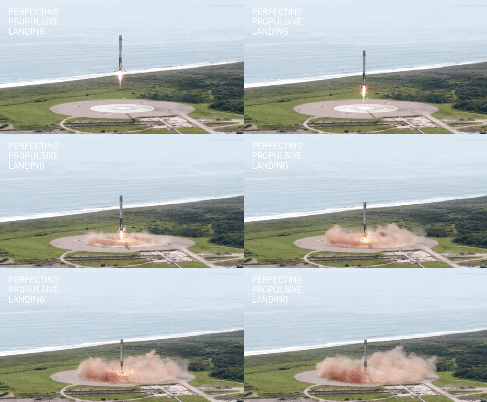
In this assignment, we will predict if the Falcon 9 first stage will land successfully. SpaceX advertises Falcon 9 rocket launches on its website with a cost of 62 million dollars; other providers cost upward of 165 million dollars each, much of the savings is due to the fact that SpaceX can reuse the first stage.

In this lab, you will perform Exploratory Data Analysis and Feature Engineering.

Falcon 9 first stage will land successfully

Several examples of an unsuccessful landing are shown here:

Most unsuccessful landings are planned. Space X performs a controlled landing in the oceans.

Objectives

Perform exploratory Data Analysis and Feature Engineering using Pandas and Matplotlib

• Exploratory Data Analysis

• Preparing Data Feature Engineering

---

Import Libraries and Define Auxiliary Functions

We will import the following libraries the lab

#Pandas is a software library written for the Python programming language for data manipulation and analysis.
import pandas as pd
#NumPy is a library for the Python programming language, adding support for large, multi-dimensional arrays and matrices, along with a large collection of high-level mathematical functions to operate on these arrays
import numpy as np
# Matplotlib is a plotting library for python and pyplot gives us a MatLab like plotting framework. We will use this in our plotter function to plot data.
import matplotlib.pyplot as plt
#Seaborn is a Python data visualization library based on matplotlib. It provides a high-level interface for drawing attractive and informative statistical graphics
import seaborn as sns

Set the style for the Seaborn plots in the latter stages of this notebook.

sns.set_style("dark")

Exploratory Data Analysis

First, let's read the SpaceX dataset into a Pandas dataframe and print its summary

df=pd.read_csv("https://cf-courses-data.s3.us.cloud-object-storage.appdomain.cloud/IBM-DS0321EN-SkillsNetwork/datasets/dataset_part_2.csv")

df.head(5)

First, let's try to see how the FlightNumber (indicating the continuous launch attempts.) and Payload variables would affect the launch outcome.

We can plot out the FlightNumber vs. PayloadMassand overlay the outcome of the launch. We see that as the flight number increases, the first stage is more likely to land successfully. The payload mass is also important; it seems the more massive the payload, the less likely the first stage will return.

sns.catplot(y="PayloadMass", x="FlightNumber", hue="Class", data=df, aspect = 5)
plt.xlabel("Flight Number",fontsize=20)
plt.ylabel("Pay load Mass (kg)",fontsize=20)
plt.show()

We see that different launch sites have different success rates. CCAFS LC-40, has a success rate of 60 %, while KSC LC-39A and VAFB SLC 4E has a success rate of 77%.

Next, let's drill down to each site visualize its detailed launch records.

TASK 1: Visualize the relationship between Flight Number and Launch Site

Use the function catplot to plot FlightNumber vs LaunchSite, set the parameter x parameter to FlightNumber,set the y to Launch Site and set the parameter hue to 'class'

sns.set_palette("bright")

# Plot a scatter point chart with x axis to be Flight Number and y axis to be the launch site, and hue to be the class value
sns.catplot(data=df, x="FlightNumber", y="LaunchSite", hue="Class")
plt.ylabel("Launch Site",fontsize=15)
plt.xlabel("Flight Number",fontsize=15)
plt.show()

Now try to explain the patterns you found in the Flight Number vs. Launch Site scatter point plots.

TASK 2: Visualize the relationship between Payload and Launch Site

We also want to observe if there is any relationship between launch sites and their payload mass.

# Plot a scatter point chart with x axis to be Pay Load Mass (kg) and y axis to be the launch site, and hue to be the class value
sns.scatterplot(data=df, x="PayloadMass", y="LaunchSite", hue="Class")
plt.show()

Now if you observe Payload Vs. Launch Site scatter point chart you will find for the VAFB-SLC launchsite there are no rockets launched for heavypayload mass(greater than 10000).

TASK 3: Visualize the relationship between success rate of each orbit type

Next, we want to visually check if there are any relationship between success rate and orbit type.

Let's create a bar chart for the sucess rate of each orbit

# HINT use groupby method on Orbit column and get the mean of Class column
df_orbitsuccess = df.groupby('Orbit').mean().reset_index()

sns.barplot(data=df_orbitsuccess, x='Orbit', y='Class')
plt.show()

Analyze the ploted bar chart try to find which orbits have high sucess rate.

TASK 4: Visualize the relationship between FlightNumber and Orbit type

For each orbit, we want to see if there is any relationship between FlightNumber and Orbit type.

# Plot a scatter point chart with x axis to be FlightNumber and y axis to be the Orbit, and hue to be the class value
sns.scatterplot(data=df, x='FlightNumber', y='Orbit', hue='Class')
plt.show()

You should see that in the LEO orbit the Success appears related to the number of flights; on the other hand, there seems to be no relationship between flight number when in GTO orbit.

TASK 5: Visualize the relationship between Payload and Orbit type

Similarly, we can plot the Payload vs. Orbit scatter point charts to reveal the relationship between Payload and Orbit type

# Plot a scatter point chart with x axis to be Payload and y axis to be the Orbit, and hue to be the class value
sns.scatterplot(data=df, x='PayloadMass', y='Orbit', hue='Class')
plt.show()

With heavy payloads the successful landing or positive landing rate are more for Polar,LEO and ISS.

However for GTO we cannot distinguish this well as both positive landing rate and negative landing(unsuccessful mission) are both there here.

TASK 6: Visualize the launch success yearly trend

You can plot a line chart with x axis to be Year and y axis to be average success rate, to get the average launch success trend.

The function will help you get the year from the date:

# A function to Extract years from the date 
year=[]
def Extract_year(date):
    for i in df["Date"]:
        year.append(i.split("-")[0])
    return year
    

df['Year'] = Extract_year('Date')

# Plot a line chart with x axis to be the extracted year and y axis to be the success rate
sns.lineplot(data=df, x='Year', y='Class')
plt.show()

you can observe that the sucess rate since 2013 kept increasing till 2020

Features Engineering

By now, you should obtain some preliminary insights about how each important variable would affect the success rate, we will select the features that will be used in success prediction in the future module.

features = df[['FlightNumber', 'PayloadMass', 'Orbit', 'LaunchSite', 'Flights', 'GridFins', 'Reused', 'Legs', 'LandingPad', 'Block', 'ReusedCount', 'Serial']]
features.head()

TASK 7: Create dummy variables to categorical columns

Use the function get_dummies and features dataframe to apply OneHotEncoder to the column Orbits, LaunchSite, LandingPad, and Serial. Assign the value to the variable features_one_hot, display the results using the method head. Your result dataframe must include all features including the encoded ones.

# HINT: Use get_dummies() function on the categorical columns
features_one_hot = pd.get_dummies(features)

features_one_hot

TASK 8: Cast all numeric columns to float64

Now that our features_one_hot dataframe only contains numbers cast the entire dataframe to variable type float64

# HINT: use astype function
features_one_hot = features_one_hot.astype('float64')

We can now export it to a CSV for the next section,but to make the answers consistent, in the next lab we will provide data in a pre-selected date range.

features_one_hot.to_csv('dataset_part\_3.csv', index=False)

Authors

Joseph Santarcangelo has a PhD in Electrical Engineering, his research focused on using machine learning, signal processing, and computer vision to determine how videos impact human cognition. Joseph has been working for IBM since he completed his PhD.

Nayef Abou Tayoun is a Data Scientist at IBM and pursuing a Master of Management in Artificial intelligence degree at Queen's University.

Change Log

Date (YYYY-MM-DD)	Version	Changed By	Change Description
2021-10-12	1.1	Lakshmi Holla	Modified markdown
2020-09-20	1.0	Joseph	Modified Multiple Areas
2020-11-10	1.1	Nayef	updating the input data

Copyright © 2020 IBM Corporation. All rights reserved.