Guide-to-cuda-q-backends.ipynb

Kernel: Python 3

# SPDX-License-Identifier: Apache-2.0 AND CC-BY-NC-4.0
#
# Licensed under the Apache License, Version 2.0 (the "License");
# you may not use this file except in compliance with the License.
# You may obtain a copy of the License at
#
# http://www.apache.org/licenses/LICENSE-2.0
#
# Unless required by applicable law or agreed to in writing, software
# distributed under the License is distributed on an "AS IS" BASIS,
# WITHOUT WARRANTIES OR CONDITIONS OF ANY KIND, either express or implied.
# See the License for the specific language governing permissions and
# limitations under the License.

Accelerating Quantum Computing: A Step-by-Step Guide to Expanding Simulation Capabilities and Enabling Interoperability of Quantum Hardware

Overview of methods of accelerating quantum simulation with GPUs

This notebook includes the following:

• Introduction to CUDA-Q through two Hello World examples using sample and observe calls.

• Guide to different backends for executing quantum circuits, emphasizing a variety of patterns of parallelization:

  • Statevector memory over multiple processors for simulation

  • Circuit sampling over multiple processors

  • Hamiltonian batching

  • Circuit cutting

  • Quantum hardware

Hello World Examples

# Uncomment and execute this cell if necessary
#!pip install cuda-quantum==0.8.0

import cudaq
from cudaq import spin
from typing import List
import numpy as np
import sys

In the first example below, we demonstrata how to define and sample a quantum kernel that encodes a quantum circuit.

# Example 1 - defining, drawing, and sampling a quantum kernel

##############################################################
#  1. Select a backend for kernel execution
cudaq.set_target("qpp-cpu")
##############################################################

##############################################################
# 2. Define a kernel function 
@cudaq.kernel
def kernel(qubit_count: int):
    # Allocate our `qubit_count` to the kernel.
    qvector = cudaq.qvector(qubit_count)

    # Apply gates to the qubit indexed by 0.
    # CUDA-Q has several built in gates beyond the few examples below
    # For a full list see https://nvidia.github.io/cuda-quantum/latest/api/default_ops.html
    z(qvector[0])
    z(qvector[0])
    s(qvector[0])
    t(qvector[0])
    s(qvector[0])
    h(qvector[0])
        
    # Apply gates to all qubits
    x(qvector)
    
    # Apply a Controlled-X gate between qubit 0 (acting as the control)
    # and each of the remaining qubits.  
    for i in range(1, qubit_count):
        x.ctrl(qvector[0], qvector[i])

    # Measure the qubits
    # If we don't specify measurements, all qubits are measured in
    # the Z-basis by default.
    mz(qvector)

##############################################################
# 3. Call the kernel function with the variable qubit_count set to 2 and sample the outcomes
qubit_count = 2
result = cudaq.sample(kernel, qubit_count, shots_count=1000)
print(result)

Now it's your turn to try it out.

Exercise 1: Edit the code below to create a kernel that produces a circuit for the GHZ state with 4 qubits

# Exercise 1 - Edit the code below to create a kernel that produces a
# circuit for the GHZ state with 4 qubits

##############################################################
#  1. Select a backend for kernel execution
cudaq.set_target("qpp-cpu")
##############################################################

##############################################################
# 2. Define a kernel function 
@cudaq.kernel
def kernel(qubit_count: int):
    # Allocate our `qubit_count` to the kernel.
    qvector = cudaq.qvector(qubit_count)

    ##############################################################
    # Edit code below
    
    # Apply a Hadamard gate to the qubit indexed by 0.
    
    
    # Apply a Controlled-X gate between qubit 0 (acting as the control)
    # and each of the remaining qubits.  

    # Measure the qubits

    # Edit code above
    ##############################################################
    
##############################################################
# 3. Call the kernel function with the variable qubit_count set to 2 and sample the outcomes
qubit_count = 4
result = cudaq.sample(kernel, qubit_count, shots_count=1000)

print(result)

The next example illustrates a few things:

• Kernels can be used to define subcircuits.

• cudaq.draw can produce ascii or LaTeX circuit diagrams

• We can define Hamiltonians with spin operators and compute expecation values with observe.

# Example 2 - Expectation value calculations

# Define a quantum kernel function to apply a CNOT gate between a control qubit and a each qubit in a list of target qubits

@cudaq.kernel
def cnot_kernel(control: cudaq.qubit, targets: cudaq.qview):
    # Apply a Controlled-X gate between qubit 0 (acting as the control)
    # and each of the remaining qubits.  
    for i in range(len(targets)):
        x.ctrl(control, targets[i])

# Define a quantum kernel function to generate a GHZ state on multpile qubits
@cudaq.kernel
def kernel(qubit_count: int):
    # Allocate our `qubit_count` to the kernel.
    control_qubit = cudaq.qubit()
    target_qubits = cudaq.qvector(qubit_count-1)

    # Apply a Hadamard gate to the qubit indexed by 0.
    h(control_qubit)
    # Apply a Controlled-X gate between qubit 0 (acting as the control)
    # and each of the remaining qubits.  
    cnot_kernel(control_qubit, target_qubits)

# Define a Hamiltonian in terms of Pauli Spin operators.
hamiltonian = spin.z(0) + 2*spin.y(1) - spin.x(0) * spin.z(1) - spin.i(2)

# Compute the expectation value given the state prepared by the kernel.
qubit_count = 3
result = cudaq.observe(kernel, hamiltonian, qubit_count, shots_count = 1000).expectation()

print(cudaq.draw(kernel, qubit_count)) 
#print(cudaq.draw('latex', kernel, qubit_count)) # Use the 'latex' option to generate LaTeX code for
print(hamiltonian)
print('<psi|H|psi> =', result)

Guide to Different Simulation Targets

The figure below illustrates a few options for accelerating statevector simulations of single quantum processor kernel executions on one CPU, one GPU, or a multi-node, multi-GPU system.

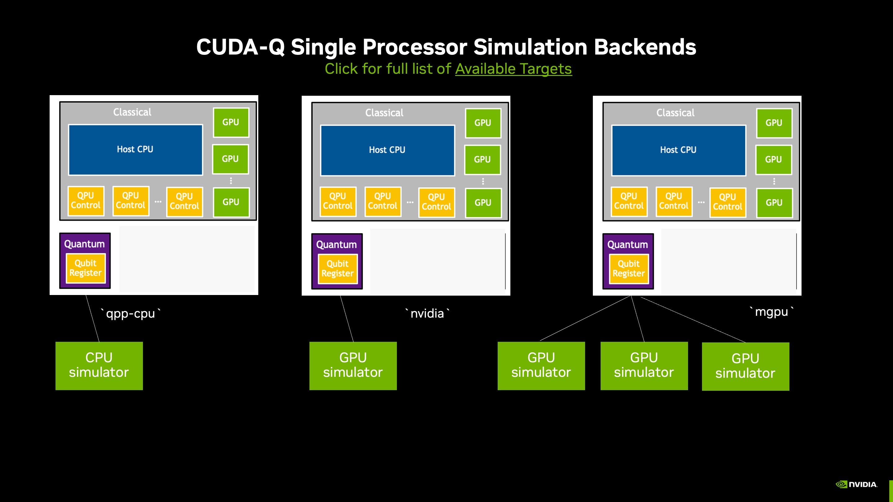
In the Hello World examples in the previous section, we saw statevector simulations of a QPU on a CPU. When GPU resources are available, we can use a single-GPU or multi-node, multi-GPU systems for fast statevector simulations. The nvidia target accelerates statevector simulations through cuStateVec library. This target offers a variety of configuration options:

• Single-precision GPU simulation (default): The default of setting the target to nvidia through the command cudaq.set_target('nvidia') provides single (fp32) precision statevector simulation on one GPU.

• Double fp64 precision on a single-GPU: The option cudaq.set_target('nvidia', option='fp64') increases the precision of the statevector simulation on one GPU.

• Multi-node, multi-GPU simulation: To run the cuStateVec simulator on multiple GPUs, set the target to nvidia with the mgpu option (cudaq.set_target('nvidia', option='mgpu,fp64')) and then run the python file containing your quantum kernels within a MPI context: mpiexec -np 2 python3 program.py. Adjust the -np tag according to the number of GPUs you have available.

Next, we'll cover a few of the ways you can organize the distribution of quantum simulations over multiple GPU processors, whether you are simulating a single quantum processing unit (QPU) or multiple QPUs.

Single-QPU Statevector Simulations

In some cases, the memory required to hold the entire statevector for a simulation exceeds the memory of a single GPU. In these cases, we can distribute the statevector across multiple GPUs as the diagram in the image below suggests.

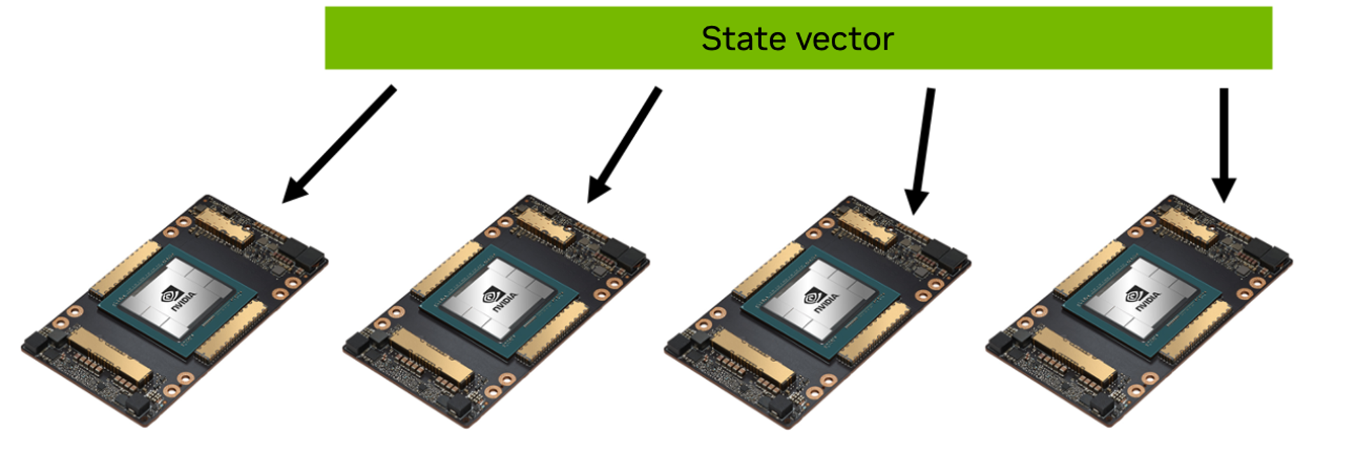
This is handled automatically within the mgpu option when the number of qubits in the statevector exceeds 25. By changing the environmental variable CUDAQ_MGPU_NQUBITS_THRESH prior to setting the target, you can change the threshold at which the statevector distribution is invoked.

Simulating Parallel QPU computaiton

Future quantum computers will accelerate performance by linking multiple QPUs for parallel processing. Today, you can simulate and test programs for these systems using GPUs, and with minimal changes to the target platform, the same code can be executed on multi-QPU setups once they are developed.

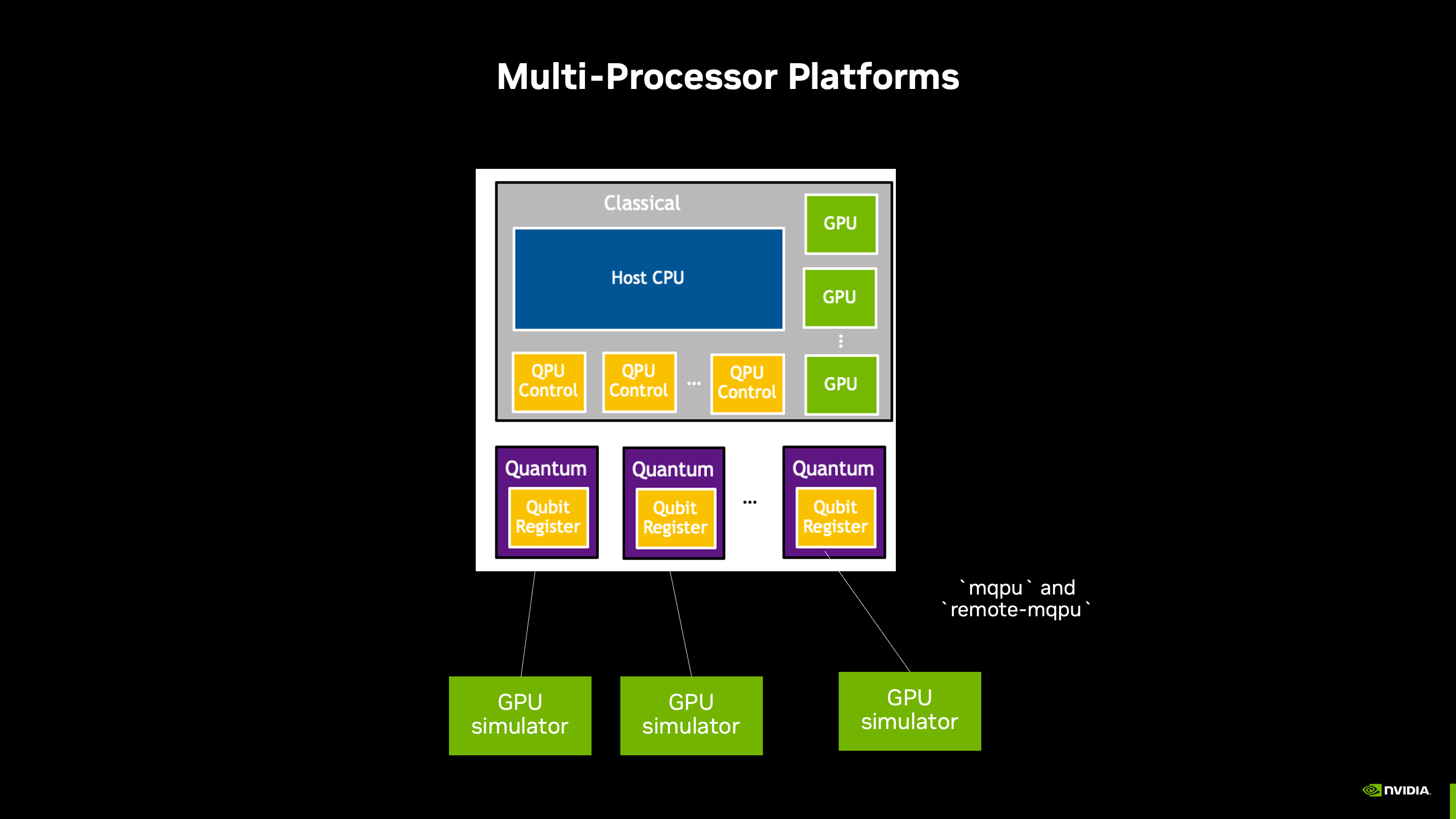
We'll examine a few multi-QPU parallelization patterns here:

• Circuit sampling distributed over multiple processors

• Hamiltonian batching

• Circuit cutting

Circuit Sampling

One method of parallelization is to sample a circuit over several processors as illustrated in the diagram below.

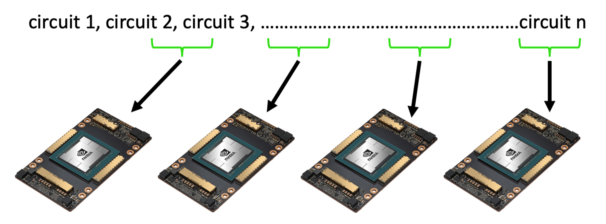
Check out the documentation for code that demonstrates how to launch asynchronous sampling tasks using sample_async on multiple virtual QPUs, each simulated by a tensornet simulator backend using the remote-mqpu target.

Hamiltonian Batching

Another method for distributing the computational load in a simulation is Hamiltonian batching. In this approach, the expectation values of the Hamiltonian's terms are calculated in parallel across several virtual QPUs, as illustrated in the image below.

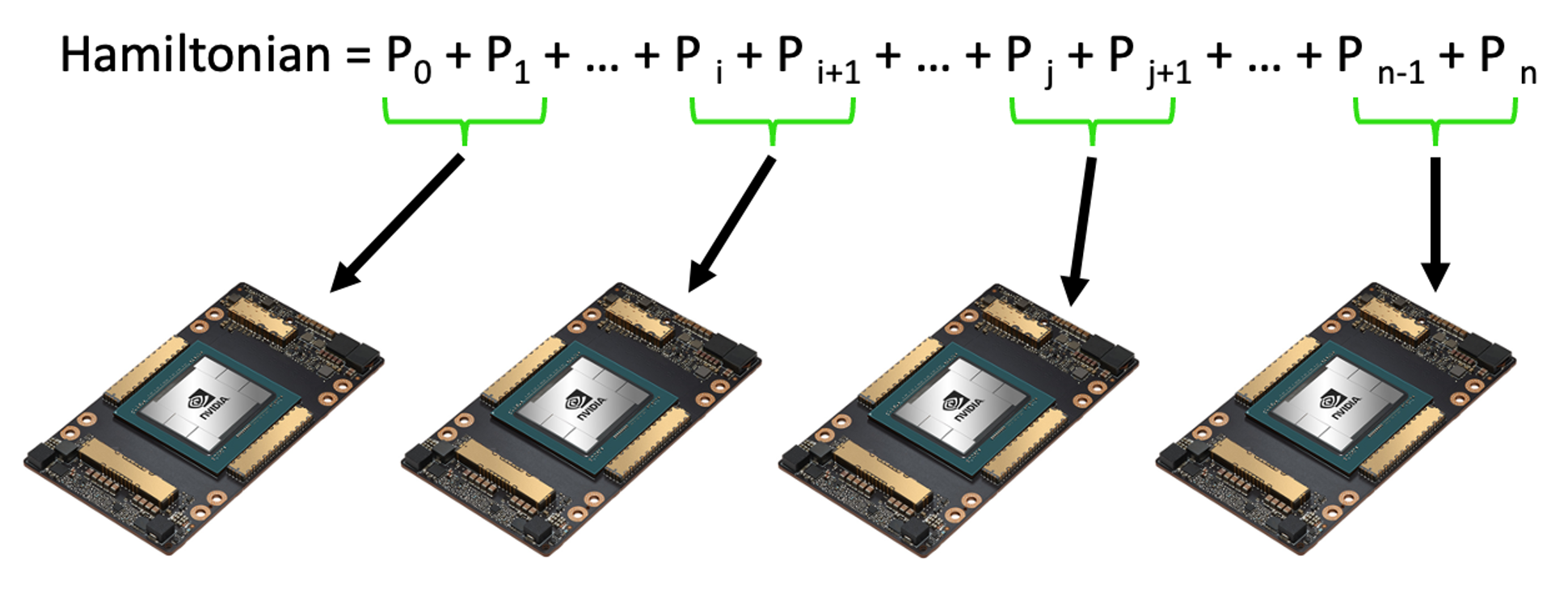
The nvidia-mqpuoption of the nvidia target along with the execution=cudaq.parallel.thread option in the observe call handles the distribution of the expectation value computations of a multi-term Hamiltonian across multiple virtual QPUs for you. Refer to the example below to see how this is carried out:

cudaq.set_target("nvidia", option="mqpu")
target = cudaq.get_target()
num_qpus = target.num_qpus()
print("Number of QPUs:", num_qpus)


# Define spin ansatz.
@cudaq.kernel
def kernel(angle: float):
    qvector = cudaq.qvector(2)
    x(qvector[0])
    ry(angle, qvector[1])
    x.ctrl(qvector[1], qvector[0])


# Define spin Hamiltonian.
hamiltonian = 5.907 - 2.1433 * spin.x(0) * spin.x(1) - 2.1433 * spin.y(
    0) * spin.y(1) + .21829 * spin.z(0) - 6.125 * spin.z(1)

exp_val = cudaq.observe(kernel,
                        hamiltonian,
                        0.59,
                        execution=cudaq.parallel.thread).expectation()
print("Expectation value: ", exp_val)

In the above code snippet, since the Hamiltonian contains four non-identity terms, there are four quantum circuits that need to be executed. When the nvidia-mqpu platform is selected, these circuits will be distributed across all available QPUs. The final expectation value result is computed from all QPU execution results.

An alternative method for orchestrating Hamiltonian batching is to use the MPI context and multiple GPUs. You can read more about this here.

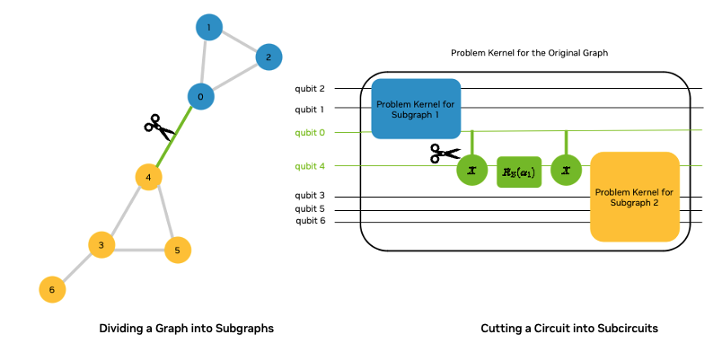
Circuit cutting

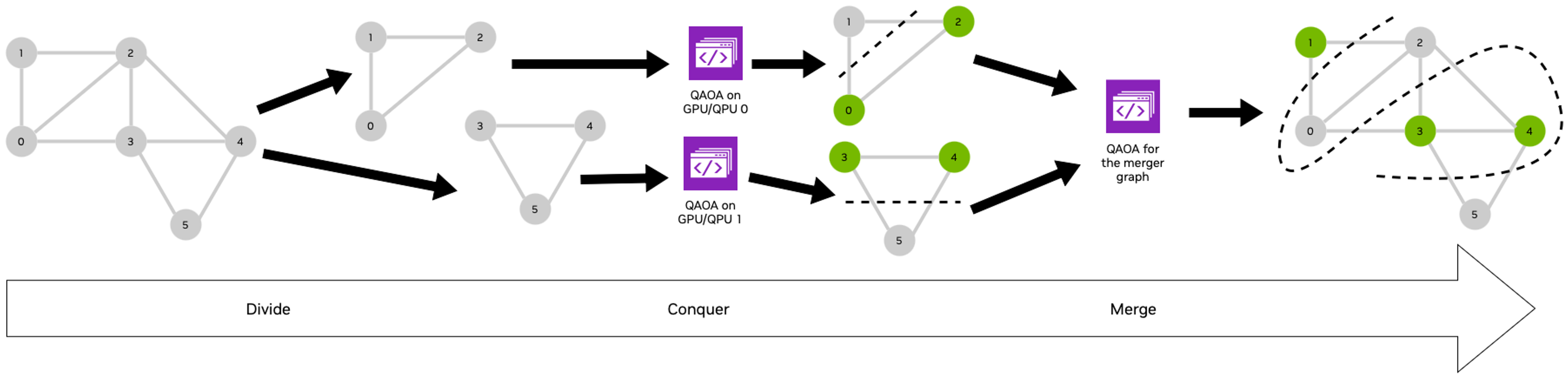
Circuit cutting is a widely used technique for parallelization. One way to conceptualize circuit cutting is through the Max Cut problem. In this scenario, we aim to approximate the Max Cut of a graph using a divide-and-conquer strategy, also known as QAOA-in-QAOA or QAOA². This approach breaks the graph into smaller subgraphs and solves the Max Cut for each subgraph in parallel using QAOA (see references such as arXiv:2205.11762v1, arxiv.2101.07813v1, arxiv:2304.03037v1, arxiv:2009.06726, and arxiv:2406:17383). By doing so, we effectively decompose the QAOA circuit for the larger graph into smaller QAOA circuits for the subgraphs.

To complete the circuit cutting, we'll need to merge the results of QAOA on the subgraphs into a result for the entire graph. This requires solving another smaller optimization problem, which can also be tackled with QAOA. You can read about that in more detail in a series of interactive labs.

This example illustrates how to use the MPI context to orchestrate running @cudaq.kernel decorated functions in parallel. Additionally, a few exercises are built into this longer example to provide some practice with the CUDA-Q commands introduced earlier in this notebook. Solutions to these exercises appear in the solutions-sc24.ipynb file, but we encourage you to first attempt the exercises out yourself.

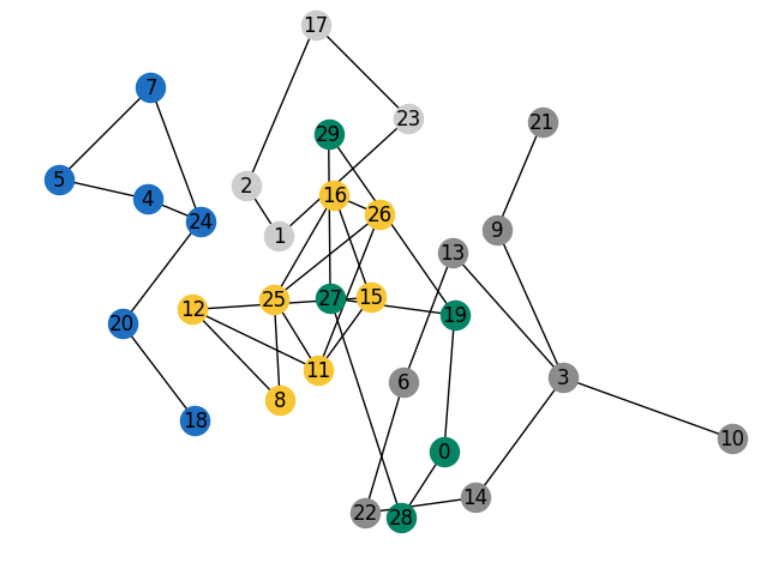
First we need to define a graph and subgraphs. Let's start with the graph drawn below.

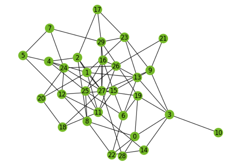
For this demonstration, we'll divide our example graph into the five subgraphs depicted below:

Execute the cell below to generate subgraphs for the divide-and-conquer QAOA.

# Identify subgraphs, separating out the edges as source and target nodes
num_subgraphs = 5 # Number of subgraphs
nodeCountList = [8,7,6,5,4] # Number of nodes in each subgraph
nodeList : List[int] = [] # List of nodes in each of the subgraphs 
edgeListSources : List[int] = [] # List of edge sources in each subgraph
edgeListTargets : List[int] = [] # List of edge targets in each subgraph

# subgraph0 data
nodeList.append([3, 6, 9, 10, 13, 14, 21, 22])
edgeListSources.append([3,3,3,3,6,6,9,14])
edgeListTargets.append([14,9,10,13,22,13,21,22])

# subgraph1 data
nodeList.append([8, 11, 12, 15, 16, 25, 26])
edgeListSources.append([8, 8, 11, 11, 11, 11, 12, 15, 16, 16, 25])
edgeListTargets.append([25, 12, 26, 25, 15, 12, 15, 16, 25, 26, 26])

# subgraph2 data
nodeList.append([4, 5, 7, 18, 20, 24])
edgeListSources.append([4, 4, 5, 7, 18, 20])
edgeListTargets.append([5, 24, 7, 24, 20, 24])

# subgraph3 data
nodeList.append([0, 19, 27, 28, 29])
edgeListSources.append([0, 0, 19, 19, 27, 27])
edgeListTargets.append([19, 28, 27, 29, 29, 28])

# subgraph4 data
nodeList.append([1, 2, 17, 23])
edgeListSources.append([1, 1, 2, 17])
edgeListTargets.append([23, 2, 17, 23])

Next, we need a helper function that will be used to map graph nodes to qubits.

# We'll create this function to rename the nodes to be sequential integers
# beginning with 0 as a way to map the graph nodes to qubits. We take this
# approach because we can't use the `.index` option for lists
# within a cudaq.kernel.
def rename_nodes(edge_src, edge_tgt, nodes):
    """ 
    Parameters
    ----------
    edges_src: List[int]
        List of the first (source) node listed in each edge of the graph, when the edges of the graph are listed as pairs of nodes
    edges_tgt: List[int]
        List of the second (target) node listed in each edge of the graph, when the edges of the graph are listed as pairs of nodes
    nodes: List[int]
        List of nodes of the graph
    
    Returns
    -------
    new_edge_src : List[int]
        List of the first (source) node listed in each edge of the graph after renaming nodes to be sequential integers beginning with 0, 
        when the edges of the graph are listed as pairs of nodes
    new_edge_tgt : List[int]
        List of the second (target) node listed in each edge of the graph after renaming nodes to be sequential integers beginning with 0, 
        when the edges of the graph are listed as pairs of nodes
    """
    new_edge_src = []
    new_edge_tgt = []
    for i in range(len(edge_src)):
        new_edge_src.append(nodes.index(edge_src[i]))
        new_edge_tgt.append(nodes.index(edge_tgt[i]))
    return new_edge_src, new_edge_tgt    

Next let's create kernels to combine into the QAOA circuit:

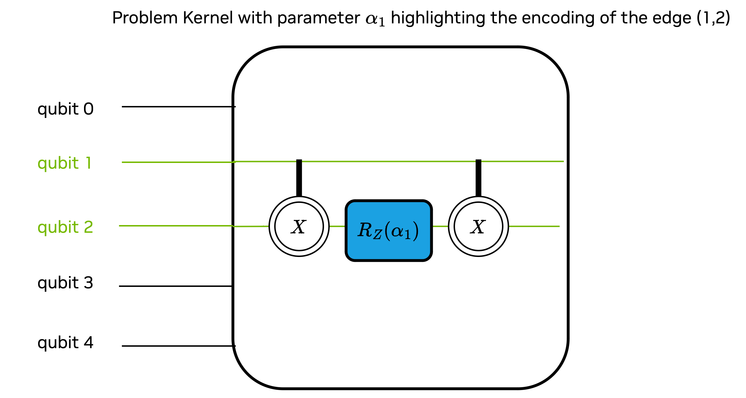
• qaoaProblem kernel adds the gate sequence depicted below for each edge in the graph

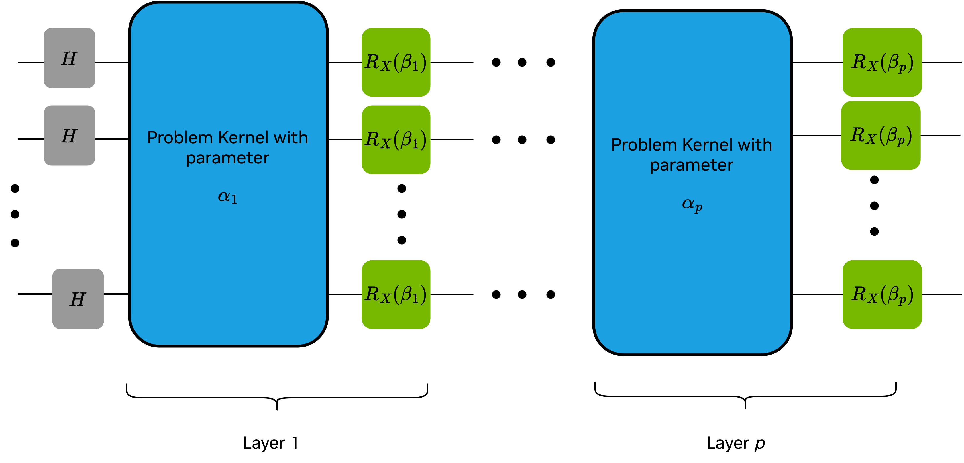
• qaoaMixer applies a parameterized rx gate to all the qubits, highlighted in green in the diagram below

• kernel_qaoa builds the QAOA circuit drawn below using the qaoaProblem and qaoaMixer

Exercise 2: The kernel_qaoa kernel has been defined for you. Your task is edit the two ###FIX_ME###s in the code below to complete the qaoaProblem and qaoaMixer kernels.

# Exercise 2 Edit the two ###FIX_ME###s in the code below. One is in `qaoaProblem` and the other is in `qaoaMixer`

# Problem Kernel
@cudaq.kernel
def qaoaProblem(qubit_0 : cudaq.qubit, qubit_1 : cudaq.qubit, alpha : float):
    """Build the QAOA gate sequence between two qubits that represent an edge of the graph
    Parameters
    ----------
    qubit_0: cudaq.qubit
        Qubit representing the first vertex of an edge
    qubit_1: cudaq.qubit
        Qubit representing the second vertex of an edge
    alpha: float
        Free variable

    """
    x.ctrl(qubit_0, qubit_1)
    ###FIX_ME###
    x.ctrl(qubit_0, qubit_1)

# Mixer Kernel
@cudaq.kernel
def qaoaMixer(###FIX_ME###):
    """Build the QAOA gate sequence that is applied to each qubit in the mixer portion of the circuit
    Parameters
    ----------
    qubit_0: cudaq.qubit
        Qubit
    beta: float
        Free variable

    """
    rx(2.0*beta, qubits)


# We now define the kernel_qaoa function which will build the QAOA circuit for our graph
@cudaq.kernel
def kernel_qaoa(qubit_count :int, layer_count: int, qubits_src: List[int], qubits_tgt: List[int], thetas : List[float]):
    """Build the QAOA circuit for max cut of the graph with given edges and nodes
    Parameters
    ----------
    qubit_count: int
        Number of qubits in the circuit, which is the same as the number of nodes in our graph
    layer_count : int
        Number of layers in the QAOA kernel
    edges_src: List[int]
        List of the first (source) node listed in each edge of the graph, when the edges of the graph are listed as pairs of nodes
    edges_tgt: List[int]
        List of the second (target) node listed in each edge of the graph, when the edges of the graph are listed as pairs of nodes
    thetas: List[float]
        Free variables to be optimized
    """
    # Let's allocate the qubits
    qreg = cudaq.qvector(qubit_count)

    # And then place the qubits in superposition
    h(qreg)
    
    # Each layer has two components: the problem kernel and the mixer
    for i in range(layer_count):
        # Add the problem kernel to each layer
        for edge in range(len(qubits_src)):
            qubitu = qubits_src[edge]
            qubitv = qubits_tgt[edge]
            qaoaProblem(qreg[qubitu], qreg[qubitv], thetas[i])
        # Add the mixer kernel to each layer
        qaoaMixer(qreg,thetas[i+layer_count])

We'll need a Hamiltonian to encode the cost function: $$H= \frac{1}{2}\sum_{(u,v)\in E} (Z_uZ_v-II),$$ where $E$ is the set of edges of the graph.

# Define a function to generate the Hamiltonian for a max cut problem using the graph G

def hamiltonian_max_cut(sources : List[int], targets : List[int]):
    """Hamiltonian for finding the max cut for the graph with edges defined by the pairs generated by sources and targets

    Parameters
    ----------
    sources: List[int]
        list of the source vertices for edges in the graph
    targets: List[int]
        list of the target vertices for the edges in the graph

    Returns
    -------
    cudaq.SpinOperator
        Hamiltonian for finding the max cut of the graph defined by the given edges
    """
    hamiltonian = 0
   
    # Since our vertices may not be a list from 0 to n, or may not even be integers,
    # we need to map the vertices to the list of integers 0 to qubit_count -1
    
    for i in range(len(sources)):
        # Add a term to the Hamiltonian for the edge (u,v)
        qubitu = sources[i]
        qubitv = targets[i]
        hamiltonian += 0.5*(spin.z(qubitu)*spin.z(qubitv)-spin.i(qubitu)*spin.i(qubitv))

    return hamiltonian

Now let's put this all together in a function that finds the the optimal parameters for QAOA of a given subgraph.

def find_optimal_parameters(qubit_src : List[int], qubit_tgt : List[int], qubit_count : int, layer_count: int, seed :int):
    """Function for finding the optimal parameters of QAOA for the max cut of a graph
    Parameters
    ----------
    qubit_src: List[int]
    qubit_tgt: List[int]
        Sources and targets defining the edges of the graph
    nodes: List[int]
        Integer labels of the nodes of the graph
    qubit_count: int
        qubit_count is the number of nodes in the graph
    layer_count : int
        Number of layers in the QAOA circuit
    seed : int
        Random seed for reproducibility of results

    Returns
    -------
    list[float]
        Optimal parameters for the QAOA applied to the given graph
    """
    
    # Each layer of the QAOA kernel contains 2 parameters
    parameter_count : int = 2*layer_count

    # Specify the optimizer and its initial parameters.
    optimizer = cudaq.optimizers.COBYLA()
    np.random.seed(seed)
    optimizer.initial_parameters = np.random.uniform(-np.pi, np.pi,
                                                     parameter_count)
    
    # Pass the kernel, spin operator, and optimizer to `cudaq.vqe`.
    optimal_expectation, optimal_parameters = cudaq.vqe(
        kernel=kernel_qaoa,
        spin_operator=hamiltonian_max_cut(qubit_src, qubit_tgt),
        argument_mapper=lambda parameter_vector: (qubit_count, layer_count, qubit_src, qubit_tgt, parameter_vector),
        optimizer=optimizer,
        parameter_count=parameter_count)

    return optimal_parameters

Before running this function in parallel, let's execute it sequentially.

# Testing the find_optimal_parameters function
layer_count = 1
seed = 123

new_src = []
new_tgt = []
optimal_parameters = []

for i in range(num_subgraphs):
    src, tgt= rename_nodes(edgeListSources[i], edgeListTargets[i], nodeList[i])
    new_src.append(src)
    new_tgt.append(tgt)
    optimal_parameters.append(find_optimal_parameters(src, tgt, nodeCountList[i], layer_count, seed))

print(optimal_parameters)

[[2.760265752934724, -1.1781480121902836], [2.863390666464872, -1.2262588372574177], [2.7568258048030376, -1.1779328954753276], [2.8169010481390853, -1.2171055596613192], [2.7488320354701976, -1.178054032241366]]

Finally, we'll need to sample the kernel_qaoa circuit with the optimal parameters to find approximate max cut solutions to each of the subgraphs.

Exercise 3: Edit the FIX_ME in the code block below to sample the QAOA circuits for each of the subgraphs using the optimal parameter found above.

# Exercise 3
# Sampling the QAOA circuits with the optimal parameters to identify an appoximate max cut of the subgraphs

shots = 10000

for i in range(num_subgraphs):
    counts = FIX_ME(kernel_qaoa, nodeCountList[i], layer_count, new_src[i], new_tgt[i], optimal_parameters[i], shots_count=shots)
    print('subgraph ',i,' has most_probable outcome = ',counts.most_probable())

That completes the "conquer" stage of the divide-and-conquer algorithm. To learn more about how the results of the subgraph solutions are merged together to get a max cut approximation of the original graph, check out the 2nd notebook of this series of interactive tutorials. For the purposes of today's tutorial we'll set that step aside and examine how we could parallelize the divide-and-conquer QAOA algorithm using CUDA-Q and MPI.

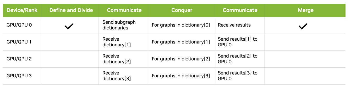
The diagram below illustrates a strategy for implementing the divide-and-conquer QAOA across 4 processors (which could be distinct GPUs or separate processes on a single GPU). The approach involves storing subgraph data in a dictionary, where the keys represent subgraph names. These dictionary keys are distributed among the 4 processors, with each processor responsible for solving the QAOA problem for the subgraphs corresponding to its assigned keys.

We've coded this strategy up in the one-step-qaoa.py file for you. The command line below executes the qaoa-divide-and-conquer.py file on 4 processors in parallel.

# Uncomment and execute this cell to install mpi4py if necessary
#%pip install mpi4py

# MPI call
# Uncomment if you have OpenMPI installed with a GPU
#print(sys.executable)
#python_path = sys.executable
#!mpiexec -np 4 --oversubscribe --allow-run-as-root {python_path} divide-and-conquer-qaoa.py

The animation below captures a small instance of a recursive divide-and-conquer QAOA running on a CPU versus a GPU in parallel. The lineplots on the top depict the error between the calculated max cut solution and the true max cut of the graph over time. The graphs on the bottom represent the max cut solutions as various subgraph problems are solved and merged together. The green graphs on the right show the parallelization of solving subgraph problems simultaneously.

Beyond Statevector Simulations

Other simulators

When using CUDA-Q on NVIDIA GPU with available CUDA runtime libraries, the default target is set to nvidia. This will utilize the cuQuantum single-GPU statevector simulator. On CPU-only systems, the default target is set to qpp-cpu which uses the OpenMP CPU-only statevector simulator.

For many applications, it's not necessary to simluate and access the entire statevector. The default simulator can be overridden by the environment variable CUDAQ_DEFAULT_SIMULATOR where tensor network, matrix product state simulators can be selected. Please refer to the table below for a list of backend simulator names along with its multi-GPU capability.

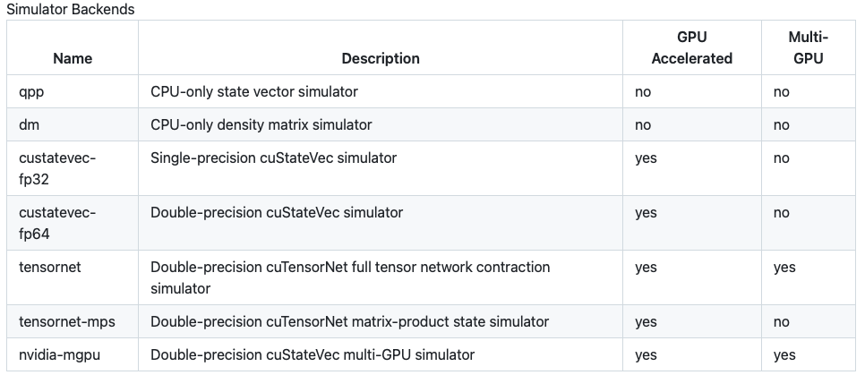
For more information about all the simulator backends available on this documentation page.

Quantum processing units

In addition to executing simulations, CUDA-Q is equipped to run quantum kernels on quantum processing units. For more information on how to execute CUDA-Q code on quantum processing units, check out the documentation.