04_quick_start_to_quantum.ipynb

Kernel: Python 3

# SPDX-License-Identifier: Apache-2.0 AND CC-BY-NC-4.0
#
# Licensed under the Apache License, Version 2.0 (the "License");
# you may not use this file except in compliance with the License.
# You may obtain a copy of the License at
#
# http://www.apache.org/licenses/LICENSE-2.0
#
# Unless required by applicable law or agreed to in writing, software
# distributed under the License is distributed on an "AS IS" BASIS,
# WITHOUT WARRANTIES OR CONDITIONS OF ANY KIND, either express or implied.
# See the License for the specific language governing permissions and
# limitations under the License.

Quick start to Quantum Computing with CUDA-Q

Lab 4 - Converge on a Solution: Write your first hybrid variational program

$\renewcommand{\ket}[1]{|{#1}\rangle} \renewcommand{\bra}[1]{\langle{#1}|}$

Labs 3 and 4 break the hybrid variational algorithm into four steps. In the first notebook (lab 3), we cover sections 1 and 2. The second notebook (lab 4) covers the remaining sections.

• Section 1: Comparing Classical Random Walks and Discrete Time Quantum Walk (DTQW)

• Section 2: Programming a variational DTQW with CUDA-Q

• Section 3: Defining Hamiltonians and Computing Expectation Values

• Section 4: Identify Parameters to Generate a Targeted Mean Value

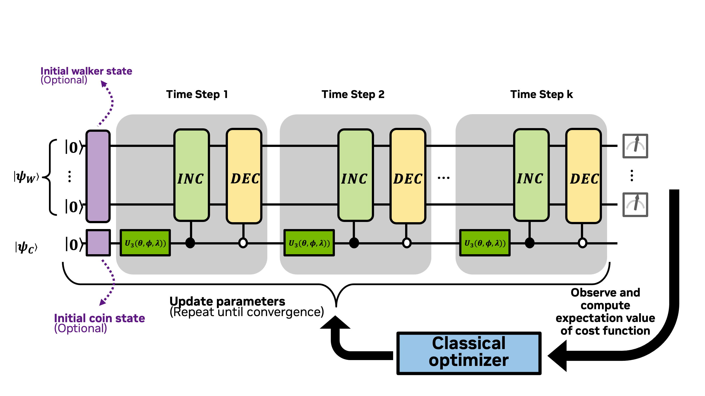
In Lab 3, we coded the parameterized kernel for the discrete time quantum walk (DTQW) using cudaq. In this notebook, we'll compute expectation values and use a classical optimizer to identify parameters to optimize a cost function, completing the coding of the diagram below:

What you'll do:

• Define and visualize Discrete Time Quantum Walks for generating probability distributions

• Add variational gates for the coin operators to create your first variational program

• Construct a Hamiltonian that can be used to compute the average of the probability distribution generated by a quantum walk

• Use a classical optimizer to identify optimal parameters in the variational quantum walk that will generate a distribution with a targeted average value

Terminology you'll use:

• Computational basis states (basis states for short)

• Probability amplitude

• Statevector

• Control and target for multi-qubit controlled-operations

• Hamiltonian

• Pauli-Z operator

CUDA-Q syntax you'll use:

• quantum kernel function decoration: @cudaq.kernel

• qubit initialization: cudaq.qvector and cudaq.qubit

• quantum gates: x, h, t, _.ctrl, cudaq.register_operation, u3

• spin operators: spin.z, spin.i

• extract information from a kernel: sample, get_state, _.amplitude, observe

• optimize parameters in a variational quantum algorithm: cudaq.optimizers

🎥 You can watch a recording of the presentation of a version of this notebook from a GTC DC tutorial in October 2025.

Let's begin by installing the necessary packages.

# Instructions for Google Colab. You can ignore this cell if you have cuda-q set up.
# Run this notebook in a CPU runtime
# Uncomment the line below and execute the cell to install cuda-q
# !pip install cudaq

import cudaq
import numpy as np
import matplotlib.pyplot as plt

We've copied over the functions from Lab 3.1 that we'll need here. Make sure you execute this cell below before continuing.

# Define a kernel on 4 qubits for the INC operation that
# maps |x> to |x+1> mod 16 

@cudaq.kernel
def INC(qubits : cudaq.qview):
    x.ctrl([qubits[3], qubits[2], qubits[1]], qubits[0])
    x.ctrl([qubits[3], qubits[2]], qubits[1])
    x.ctrl(qubits[3], qubits[2])
    x(qubits[3])
    

# Define a kernel on 4 qubits for the DEC operation that
# maps |x> to |x-1> mod 16 

@cudaq.kernel
def DEC(qubits : cudaq.qview):
    x(qubits[3])
    x.ctrl(qubits[3], qubits[2])
    x.ctrl([qubits[3], qubits[2]], qubits[1])
    x.ctrl([qubits[3], qubits[2], qubits[1]], qubits[0])

---

Section 3 Defining Hamiltonians and Computing Expectation Values

(Sections 1 and 2 can be found in Lab 3)

A significant challenge in quantum computing is the efficient encoding of classical data into quantum states that can be processed by quantum hardware or simulated on classical computers. This is particularly crucial for many financial applications, where the first step of a quantum algorithm often involves efficiently loading a probability distribution. For instance, to enable lenders to price loans more accurately based on each borrower's unique risk profile, it is essential to estimate individual loan risk distributions (such as default and prepayment) while accounting for uncertainties in modeling and macroeconomic factors. Efficiently implementing this process on a quantum computer requires the ability to load a log-normal or other complex distribution into a quantum state (Breeden and Leonova).

Financial markets exhibit complex probability distributions and multi-agent interactions that classical models struggle to capture efficiently. Quantum walks can be used to generate probability distributions of market data. The quantum walk approach offers:

• Flexible modeling of price movements

• Better representation of extreme events compared to classical methods

• Ability to capture asymmetric return distributions (Backer et al).

The Problem

This tutorial explores how to load a probability distribution with a given property (in this case, a fixed mean) into a quantum state. By following this example, you will gain the essential knowledge needed to comprehend more sophisticated algorithms, such as the multi-split-step quantum walks (mSSQW) method, as described by Chang et al. The mSSQW technique can be employed to load a log-normal distribution, which is useful for modeling the spot price of a financial asset at maturity.

Pedagogical Remark: The reason why we chose to examine the coarser problem of generating a distribution with a targeted mean as opposed to generating a targeted distribution itself (as in Chang et al.) is that by considering the mean of the distribution we can introduce the concept of expectation value of a Hamiltonian which is central to many variational algorithm applications in chemistry, optimization, and machine learning.

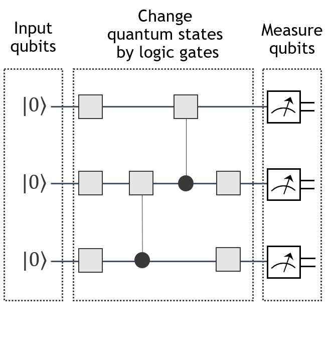
Let's begin by examining the final step in the quantum program template, which involves taking measurements and interpreting the results:

Up to this point, for this step of the quantum program, we utilized cudaq.get_state and cudaq.sample to read out a statevector from the quantum kernel. However, this approach is not always practical, especially considering that the dimension of the statevector scales exponentially with the number of qubits. For example, describing the statevector for $100$ qubits would require storing $2^{100}$ amplitudes, which is extremely memory-intensive. In many quantum algorithms, we do not need a complete description of the statevector; instead, partial information like an "average" value often suffices. This is where the concept of expectation value comes in.

Illustrative Example of Expectation Value

Before we delve into our DTQW example, let's make this idea of "average" value of a quantum state more explicit by considering a specific example.

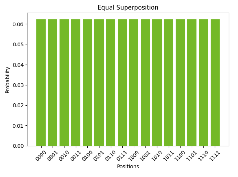
Take the quantum state $\ket{\psi} = \sum_j\alpha_j\ket{j}$, where $\alpha_j = \frac{1}{4}$ for all $j\in\{0, \cdots 15\}$. The probability amplitudes for the computational basis states of this example are graphed below:

Expectation Values

We can think of this as a probability distribution of a random variable and compute the expectation value (i.e., average or mean). Graphically, we can determine that the expectation value is the position halfway between $\ket{7}$ and $\ket{8}$ (i.e., between the states $\ket{0111}$ and $\ket{1000}$). Analytically, we'd find this by computing $\sum^{15}_{j=0} p_j i$, where $p_j$ is the probability of measuring the state $\ket{j}$. In this example we'd get $\sum^{15}_{j=0} p_j j = \frac{1}{16}\sum_{j=0}^{15}j = 7.5.$

Let's look into how, in general, we can deduce the expectation value $\sum^{15}_{j=0} p_j j$ from a state $\ket{\phi} = \sum_j\alpha_j\ket{j}$. We know that $|\alpha_j|^2 = p_j$, by definition of the probability amplitudes. Therefore, to complete the computation, we need an operation to translate from $\ket{j}$ to $j$.

This is where the Hamiltonian comes in. We won't formally define a Hamiltonian in its full generality here (you can read more about Hamiltonians in Scott Aaronson's lecture notes). For this tutorial, we will consider a Hamiltonian to be a $16\times 16$ matrix that operates on a $4$-qubit quantum state through matrix multiplication. This matrix has certain additional properties, which we will not focus on for now. For the purposes of this tutorial, all you need to know is that $H$ has the properties:

• $H(\ket{j}) = j\ket{j}$ for $j \in \{0,1,\cdots, 15\}$

• $H$ is linear, that is $H(c\ket{\psi}+d\ket{\phi}) = cH(\ket{\psi})+dH(\ket{\phi})$ for $c,d\in\mathbb{C}$ and states $\ket{\psi}$ and $\ket{\phi}$.

We've left the explicit formula for $H$ in the optional box below. But assuming that we have such an operation, then we can define and denote the expectation value of this Hamiltonian with respect to a state $\phi$ as $$\bra{\phi}H\ket{\phi} \equiv \ket{\phi}^\dagger H(\ket{\phi}),$$ where the notation $\bra{\phi}$ is read as "bra phi" and comes from the bra-ket notation. It represents the conjugate transpose of the ket, $\ket{\phi}$. In other words, bra-$\phi$ ($\bra{\phi}$) is equal to $\ket{\phi}^\dagger$. Placing $\bra{\phi}$ next to $H(\ket{\phi})$ in the equation above represents the action of taking the dot product of $\bra{\phi}$ with $H(\ket{\phi})$.

Let's compute $$\bra{\psi}H\ket{\psi},$$ for the equal superposition state $\ket{\psi} = \sum_j\frac{1}{4}\ket{j} = \frac{1}{4}\begin{pmatrix}1 \\ 1\\ \vdots \\ 1 \end{pmatrix},$ graphed above. By our choice of $H$ and its linearity, we get that

$$H\ket{\psi} = H(\sum_{j=0}^{15}\frac{1}{4}\ket{j}) = \frac{1}{4}\sum_{j=0}^{15}H(\ket{j}) = \frac{1}{4}\sum_{j=0}^{15}j(\ket{j})= \frac{1}{4}\begin{pmatrix} 0 \\ 1 \\ 2 \\ \vdots \\ 15 \end{pmatrix}.$$

Next combining this with $\bra{\psi}$ via a dot product, we get

$$\bra{\psi}H\ket{\psi} = \frac{1}{4}\begin{pmatrix}1 & 1& \cdots & 1\end{pmatrix} \frac{1}{4}\begin{pmatrix} 0 \\ 1 \\ 2 \\ \vdots \\ 15 \end{pmatrix} = \frac{1}{16}\begin{pmatrix}1 & 1& \cdots & 1\end{pmatrix}\begin{pmatrix} 0 \\ 1 \\ 2 \\ \vdots \\ 15 \end{pmatrix} = \frac{1}{16}(0+1+2+\cdots + 15) = \frac{1}{16}\sum_{j=0}^{15} j = 7.5,$$

which is exactly the expectation value that we found analytically at the beginning of this section.

Optional: The particular Hamiltonian that we need is the one that has the property $H\ket{j} = j\ket{j}$. In other words, the computational basis states are eigenvalues of the Hamiltonian and the eigenvalue of $\ket{j}$ is $j$. The Hamiltonian that has this property is $$H = \sum_{j=0}^{15}j\ket{j}\bra{j},$$ where $\ket{j}\bra{j}$ is the matrix product of $\ket{j}$ with $\bra{j}$. A more useful formulation of $H$ is $$H =\sum_{j=0}^{15}j\ket{j}\bra{j} = 4(I-Z_0) + 2(I-Z_1) + (I-Z_2) + \frac{1}{2}(I-Z_3) = 7.5I- (4Z_0 + 2 Z_1 + Z_2 +\frac{1}{2}Z_3),$$ where $I$ is the identity matrix and $Z_j$ is the $16\times16$-dimensional matrix which applies the $Z = \begin{pmatrix} 1 & 0 \\ 0 & -1\end{pmatrix}$ to the $j^{th}$ qubit and holds all other qubits constant. For example applying $Z_2$ to the state $\ket{1111}$ results in $-\ket{1111}$ and $Z_2$ applied to $\ket{1011}$ is $\ket{1011}$. With some matrix algebra, you can verify the following equality holds for $j\in \{0,1,\cdots, 15\}$: $$H\ket{j} = 7.5I\ket{j}- 4Z_0\ket{j} - 2 Z_1\ket{j} - Z_2\ket{j} -\frac{1}{2}Z_3\ket{j} = j\ket{j}.$$

Computing Expectation Values with observe

The observe function is used to compute expectation values of Hamiltonians. Suppose that the state $\ket{\psi}$ is defined by a cudaq.kernel called my_kernel, and $H$ is a Hamiltonian stored as a cudaq.operator, named my_hamiltonian. We can compute the expectation value $\bra{\psi}H\ket{\psi}$ using observe(my_kernel, my_hamiltonian).expectation(). For observe to work, the kernel shouldn't contain any measurements of the state of interest — otherwise, the state of the kernel would have collapsed to one of the basis states. We can store $H$ as a cudaq.operator using cudaq.spin.z and cudaq.spin.i along with + and scalar multiplication *. Let's walk through computing the expectation value for a probability distribution represented by a quantum state in the code block below.

# Computing expectation value of an equal superposition state

# Set the number of qubits
num_qubits = 4

# Define a kernel for the state |psi> = 1/4(|0000> + |0001> + ...+ |1111>)
@cudaq.kernel
def equal_superposition(num_qubits : int):
    """ Apply gates to the qubits to prepare the GHZ state
    Parameters
        num_qubits : int Number of qubits
    """
    # Edit the code below this line
    qubits = cudaq.qvector(num_qubits)
    for i in range(len(qubits)):
        h(qubits[i])

# Define the Hamiltonian
position_hamiltonian =  7.5*cudaq.spin.i(0) - 4*cudaq.spin.z(0)-2*cudaq.spin.z(1)-cudaq.spin.z(2)-0.5*cudaq.spin.z(3)

# Compute the expectation value
expectation_value = cudaq.observe(equal_superposition, position_hamiltonian, num_qubits).expectation()

print(expectation_value)

7.5

As anticipated, the expectation value of the equal superposition state is computed to be 7.5. In this section we introduced ideas that are essential for many other applications of variational quantum algorithms. In particular, we introduced the Hamiltonian $H$ for computing the average value of a quantum state if we identify the computational basis states with integers. We also demonstrated how to compute the expectation value of the Hamiltonian applied to a quantum state $\bra{\psi}H\ket{\psi}$ using the observe command. In the next section, we'll apply all of this to our DTQW problem.

Expectation value of a DTQW

We are now prepared to apply what we've learned to the problem of finding a Discrete-Time Quantum Walk (DTQW) that yields a probability distribution with a specific mean. Let's aim to generate a distribution from a quantum walk with a mean of $3$. In the code block below, you'll find a parameterized kernel for the DTQW based on the code that we developed in Lab 3. We've just added a flag so that we both sample and compute expectation values with the kernel.

Do your best to adjust the parameter values to achieve a state with an average close to $3$. It's challenging, isn't it? There are just so many combinations of parameter values to experiment with!

# Set a variable for the number of time steps
num_time_steps = 6

# Pick your favorite values
theta = np.pi/2    #CHANGE ME
phi = np.pi/2     #CHANGE ME  
lam = 0.0        #CHANGE ME

# Set the number of position qubits
num_qubits = 4

@cudaq.kernel()
def measure(qubits : cudaq.qview):
    mz(qubits)

@cudaq.kernel()
def DTQW_for_expectation_value_computation(num_qubits: int, parameters : list[float], num_time_steps : int, with_measurement: int):
    walker_qubits = cudaq.qvector(num_qubits)
    coin_qubit = cudaq.qvector(1)
    
    theta = parameters[0]
    phi = parameters[1]
    lam = parameters[2]

    # Initial walker state |9> = |1001> for possibly faster convergence
    #x(walker_qubits[3])
    #x(walker_qubits[2])
    
    # initial coin state
    h(coin_qubit[0])
    
    #for i in range(1, num_qubits):
    #    x.ctrl(walker_qubits[0], walker_qubits[i])
    
    # Flip the coin num_time_steps and shift the walker accordingly
    for _ in range(num_time_steps):
        
        # One quantum walk step
        # Coin operation F=u3
        u3(theta, phi, lam, coin_qubit)
    
        # Walker's position change 
        # Shift right (S+) when the coin is |1>
        cudaq.control(INC, coin_qubit[0], walker_qubits)
    
        # Shift left (S-) when the coin is |0>

        x(coin_qubit[0])
        cudaq.control(DEC, coin_qubit[0], walker_qubits)
        x(coin_qubit[0])
    
    if (with_measurement==1):
        # Measure walker qubits
        measure(walker_qubits)
        
    
# Sample the kernel for the quantum walk
result_aiming_for_mean_of_3 = cudaq.sample(DTQW_for_expectation_value_computation, num_qubits, [theta, phi, lam], num_time_steps, 1, shots_count=10000)
print('sampling results with the coin qubit:', result_aiming_for_mean_of_3)


# Define a function to draw the histogram of the results ignoring the coin qubit

def plot_results_without_coin_qubit(result, num_qubits):
    # Initialize the dictionary with all possible bit strings of length 4 for the x axis
    result_dictionary = {}

    # Generate all possible bit strings of length num_qubits
    for i in range(2**num_qubits):
        bitstr = bin(i)[2:].zfill(num_qubits)
        result_dictionary[bitstr] = 0
    
    # Update the results dictionary of results from the circuit sampling
    for k,v in result.items():
        result_dictionary[k] = v

    # Convert the dictionary to lists for x and y values
    x = list(result_dictionary.keys())
    y = list(result_dictionary.values())

    # Create the histogram
    plt.bar(x, y, color='#76B900')

    # Add title and labels
    plt.title("Sampling of the DTQW")
    plt.xlabel("Positions")
    plt.ylabel("Frequency")

    # Rotate x-axis labels for readability
    plt.xticks(rotation=45)

    # Show the plot
    plt.tight_layout()
    plt.show()

# Draw the histogram of the results after one step
plot_results_without_coin_qubit(result_aiming_for_mean_of_3, num_qubits)

# Compute the expectation value
exp_value = cudaq.observe(DTQW_for_expectation_value_computation, position_hamiltonian, num_qubits, [theta, phi, lam], num_time_steps,0).expectation()
print('The expectation value <ψ|H|ψ>  using parameters ({:.6f}, {:.6f}, and {:.6f}), is {} '.format(theta, phi, lam, exp_value))

sampling results with the coin qubit: { 0000:1250 0010:1275 0100:5279 0110:283 1100:318 1110:1595 }

The expectation value <ψ|H|ψ>  using parameters (1.570796, 1.570796, and 0.000000), is 5.125000000000002 

---

Section 4 Identify Parameters to Generate a Targeted Mean Value

We have now arrived at the need for the variational quantum algorithm (see the diagram below). We can initialize the kernel with some parameter values, and then turn the problem over to a classical optimizer to search for new parameter values that minimize a cost function (sometimes referred to as an error function). In our case we want to minimize the difference between $\bra{\psi_W} H\ket{\psi_W}$ and our targeted mean of $3$. For the cost function, we'll use the mean square error (MSE) as our metric for closeness between the expectation value and the targeted mean.

The code block below defines the cost function and creates a list to record its values at each iteration of the loop.

# Create a list to store the cost values from each iteration of the variational algorithm
cost_values = []

# Compute the cost for a given set of parameters
def cost(parameters):
    """Returns the MSE between the targeted mean of 3 and the expectation value of the DTQW as our cost,
    which we want to minimize. The cost for the given parameters is stored in the cost_values list.
    Parameters
        parameters : list[float] The parameters to be optimized
    Returns
        cost_val : float The cost value
    """
    # Compute the expectation value
    expectation_value = cudaq.observe(DTQW_for_expectation_value_computation, position_hamiltonian, num_qubits, parameters, num_time_steps, 0, shots_count = 50000).expectation()
    # Compute the cost value
    cost_val = np.sqrt((expectation_value-3)**2)
    cost_values.append(cost_val)
    return cost_val

Below we use our built-in optimization suite (cudaq.optimizers) to minimize the cost function. Specifically, we will select the gradient-free Nelder Mead classical optimization algorithm.

# Define a CUDA-Q optimizer
optimizer = cudaq.optimizers.NelderMead()

# Set initial parameter values
optimizer.initial_parameters = [theta, phi, lam]

# Optimize the cost function
# The optimizer will try to minimize the cost function defined above
result = optimizer.optimize(dimensions=3, function=cost) #dimensions is the number of parameter values

print('The minimal cost found is ',result[0])
print('The optimized parameters are ',result[1])

The minimal cost found is  3.999999999981796e-05
The optimized parameters are  [2.1272394709128655, 2.3922666219387034, -0.38655941838953967]

Let's plot the cost values for each iteration of the variational algorithm to see the convergence.

# Plotting how the value of the cost function decreases during the minimization procedure.
plt.title("Convergence of the Variational Quantum Algorithm")
x_values = list(range(len(cost_values)))
y_values = cost_values

plt.plot(x_values, y_values)

plt.xlabel("Iterations")
plt.ylabel("Cost Value")

Text(0, 0.5, 'Cost Value')

Finally, let's use the optimal parameters to carry out the DTQW to verify that we have generated a probability distribution with a mean close to 3.

optimal_parameters = result[1]
result_optimized = cudaq.sample(DTQW_for_expectation_value_computation, num_qubits, optimal_parameters, num_time_steps, 1, shots_count=10000)
print('sampling results with the coin qubit:', result_optimized)

# Draw the histogram of the results after one step
plot_results_without_coin_qubit(result_optimized, num_qubits)

# Compute the expectation value
exp_value = cudaq.observe(DTQW_for_expectation_value_computation, position_hamiltonian, num_qubits, optimal_parameters, num_time_steps,0).expectation()
print('The expectation value  <ψ|H|ψ>  is ',exp_value)

sampling results with the coin qubit: { 0000:1576 0010:6278 0100:1280 0110:1 1010:1 1100:75 1110:789 }

The expectation value  <ψ|H|ψ>  is  2.9986959931162414

---

Completion of the Quick Start to Quantum Computing Series

Congratulations! You've successfully written your first variational quantum algorithm. You're now prepared to explore more advanced examples and applications.

Additional Challenges and Exercises

To further develop your skills, consider the following problems:

1. Parameterized DTQW: Modify the existing DTQW code to incorporate different parameters in the coin flip operation u3 at each step. In other words each step of the DTQW might have a different coin operator. You can build upon the code developed in Lab 3 and 4.

2. Targeted Distribution Generation: Adapt the variational algorithm to generate a targeted distribution. To do this, you will need to sample the distribution at each stage and use the mean square error between the sampled distribution and the targeted distribution as your cost function. Hint: For this problem, you will use the sample command instead of the observe command and you will not need to define a Hamiltonian.

3. Varying the quantum walk: Consider variations to the DTQW by introducing an additional coin flip in between steps right and left (i.e., between the controlled-INC and controlled-DEC operations).

The animation below demonstrates what is possible by solving problems 1-3 above to model financial data:

Future Directions and Resources

Now that you have a solid foundation in variational quantum algorithms, you can explore more advanced topics and applications, including:

• Multi-split-step quantum walk for financial data: Apply the variational quantum algorithm template to generate probability distributions for financial data. You can learn more about this example in notebooks 1 and 2 of the CUDA-Q Academic Quantum Applications to Finance series.

• Quantum Approximate Optimization Algorithm (QAOA): Learn about QAOA, circuit cutting, and GPU acceleration as applied to the max cut optimization problem.

• Variational Quantum Eigensolver (VQE): Discover how VQE can be used to find the ground state of a quantum system.

• Hybrid quantum neural networks: Explore the intersection of quantum computing and machine learning.

To take your quantum computing skills to the next level, consider learning about accelerating quantum computing and expanding simulation capabilities. The Accelerating Quantum Computing: A Step-by-Step Guide provides a comprehensive resource to help you achieve this goal.