Path: blob/master/2019-spring/slides/12_high_dim_viz_and_wrap_up.ipynb
2735 views
DSCI 100 - Introduction to Data Science
Lecture 12 - Visualizing high dimensional data & Data Science wrap-up
2019-04-04
Output of K means multivariate clustering from tutorial
Output of K means multivariate clustering from tutorial
we can look at total within sum of squares (but really only useful for comparing models)
we can look at the ratio of between sum of squares / total sum of squares
if very small, then there are no discernable clusters
if 100, then each point is its own cluster
neither of these are very intuitive (at least to me)
What is intuitive?
Visualization! A picture says 1000 words!
t-sne
a popular dimensonality reduction algorithm useful for visualizing multi-dimensional data sets
no "model" given from t-sne (only works to visualize the data you currently have)
see links in worksheet for more details about the specifics of the algorithm if you are interested
t-sne visualization of gene expression data from cells in a region of the brain
each data point in this picture corresponds to a single brain cell for which we have the expression level measurements for thousands of genes.

source: Cembrowski, M.S., Wang, L., Lemire, A., DiLisio, S.F., Copeland, M., Clements, J., Spruston, N. The subiculum is a patchwork of discrete subregions. eLife 7, doi:10.7554/eLife.37701, 2018.
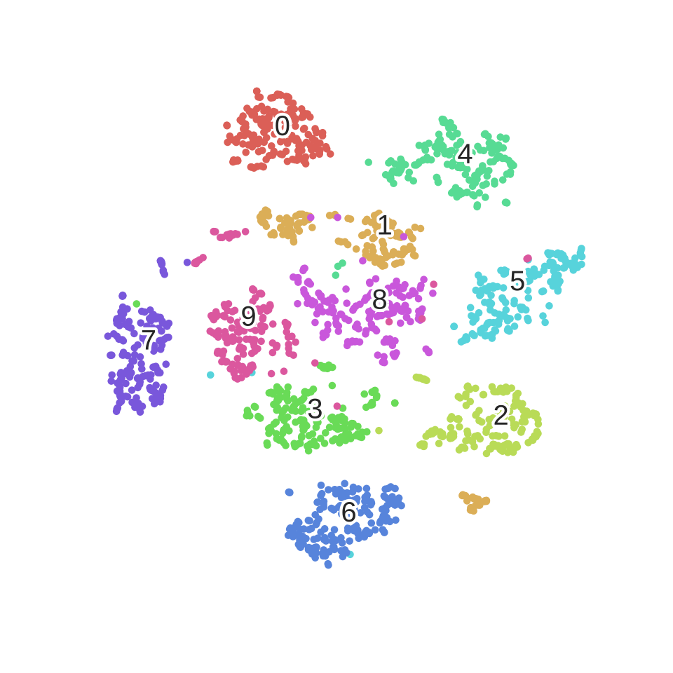
t-sne visualization of hand-written digits data set overlaid with class identification
each data point is an image of a handwritten digit for which we have 784 pixel values
COURSE EVALUATIONS!
Data Science wrap-up
In January, we started with this Gif

And we laid out these goals and this path:
High-level goals of this course:
Learn how to use reproducible tools (Jupyter + R) to do data analysis
Learn how to solve 3 common problems in Data Science
Problems we will focus on:
Predict a class/category for a new observation/measurement (e.g., cancerous or benign tumour)
Predict a value for a new observation/measurement (e.g., 10 km race time for a 35 year old with a BMI of 25).
Find previously unknown/unlabelled subgroups in your data (e.g., products commonly bought together on Amazon)
Another way to think of what we did in this course:

source: R for Data Science by Grolemund & Wickham
Where to from here
you learned a lot in this course!
many of you are asking for more Data Science (yeah!)
so here's a list of some UBC courses of interest you might want to take:
CPSC 330 - Applied Machine Learning (Instructor coming to give a sneak peak today)
outside of classes, I can recommend reading An Introduction to Statistical Learning and the John Hopkins Coursera Data Science courses
Thank-you and it's been a blast!