GitHub Repository: UBC-DSCI/dsci-100-assets
Path: blob/master/2021-spring/slides/03_wrangling.ipynb
²⁰⁵¹ views

Kernel: R

DSCI 100 - Introduction to Data Science

Lecture 3 - Wrangling to get tidy data

Credit to Jenny Brian's slides and Garrett Grolemund's tidying example

While you wait... enjoy this plot of the mtcars data set from the new {ggbernie} R package 😂:

Housekeeping

Quiz 1 will be February 11th during the tutorial time for your registered section (i.e., in class)
- 45 mins
- covers all the material from weeks 1 - 4 (but none of the optional web scraping is included)
- open book (but not collaborative)
- will be served on Canvas.
  - Make sure you have either Chrome or Firefox. Safari has been known to have trouble loading images and math.
- we will work on projects after
- practice questions will be posted -- make sure you can access the quiz on Canvas
- Invigilate using Zoom (see upcoming Canvas post "Information about the quizzes" for details) -- make sure you can use Zoom with camera on your personal device
You should see a grade for worksheet 1 and 2 on Canvas (unless you registered late)
We are working in our project groups today (different from the breakout room groups)
- Group contracts due Jan 30

Reminder

Where are we? Where are we going?

image source: R for Data Science by Grolemund & Wickham

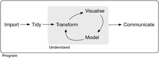
Data Wrangling!

image: Medium

In the real world, when you get data, it's usually very messy
- inconsistent format (commas, tabs, semicolons, missing data, extra empty lines)
- split into multiple files (e.g. yearly recorded data over many years)
- corrupted files, custom formats
when you read it successfully into R, it will often still be very messy

you need to make your data "tidy"

What is Tidy Data?

Illustrations from the Openscapes blog Tidy Data for reproducibility, efficiency, and collaboration by Julia Lowndes and Allison Horst"

Like families...

Comparison of work benches:

Friends with similar tools:

Easier for automation & iteration!

And it makes all other tidy datasets seem more welcoming!

So make friends with tidy data!

Examples of Tidy(?) Data

...here is the same data represented in a few different ways. Let's vote on which are tidy!

Tuberculosis data

This data is tidy. True or false?

country	year	rate
Afghanistan	1999	745/19987071
Afghanistan	2000	2666/20595360
Brazil	1999	37737/172006362
Brazil	2000	80488/174504898
China	1999	212258/1272915272
China	2000	213766/1280428583

False. Multiple variables are stored in one column.

the rate column is a combination of the number of cases and population each cell (row, column pair) does not correspond to a single value

Tuberculosis data

This data is tidy. True or false?

country	cases (year=1999)	cases (year=2000)
Afghanistan	745	2666
Brazil	37737	80488
China	212258	213766

country	population (year=1999)	population (year=2000)
Afghanistan	19987071	20595360
Brazil	172006362	174504898
China	1272915272	1280428583

False. A single observational unit is stored in multiple tables.

Here we have data values about a single type of observational unit spread out over multiple tables. These tables are split up by the number of cases of tuberculosis and the population of each country, so that each represents a single each row is not a single observation

Tuberculosis data

This data is tidy. True or false?

| country | 1999 | 2000 | |---------|-------|-------| | Afghanistan | 745 | 2666 | |Brazil |37737 | 80488 | | China | 212258 | 213766 |

False. Column headers are values, not variable names.

Here we see the columns headers are values (the year) not variable names. This common type of messy dataset is tabular data designed for presentation, where variables form both the rows and columns, and column headers are values, not variable names.

each column does not corresponds to a single variable since year is across the top

Tuberculosis data

This data is tidy. True or false?

country	year	key	value
Afghanistan	1999	cases	745
Afghanistan	1999	population	19987071
Afghanistan	2000	cases	2666
Afghanistan	2000	population	20595360
Brazil	1999	cases	37737
Brazil	1999	population	172006362
Brazil	2000	cases	80488
Brazil	2000	population	174504898
China	1999	cases	212258
China	1999	population	1272915272
China	2000	cases	213766
China	2000	population	1280428583

False. Variables are stored in both rows and columns. It has variables in individual columns (country, year), and across rows (population, cases) in the "key" column

each row does not corresponds to a single observation, each column does not corresponds to a single variable, and each cell (row, column pair) does not correspond to a single value

Tuberculosis data

This data is tidy. True or false?

country	year	cases	population
Afghanistan	1999	745	19987071
Afghanistan	2000	2666	20595360
Brazil	1999	37737	172006362
Brazil	2000	80488	174504898
China	1999	212258	1272915272
China	2000	213766	1280428583

each row corresponds to a single observation,
each column corresponds to a single variable, and
each cell (row, column pair) correspond to a single value

Tools for tidying:

tidyverse package functions from:
- dplyr package (select, filter, mutate, group_by, summarize)
- tidyr package (pivot_longer, pivot_wider)
- purrr package (map_df)

Demo Time!

In [2]:

library(tidyverse)
library(palmerpenguins)
options(repr.matrix.max.rows = 6)

Out[2]:

── Attaching packages ───────────────────────────────────────────────────────────────── tidyverse 1.3.0 ──

✔ ggplot2 3.3.2     ✔ purrr   0.3.4
✔ tibble  3.0.4     ✔ dplyr   1.0.2
✔ tidyr   1.1.2     ✔ stringr 1.4.0
✔ readr   1.4.0     ✔ forcats 0.5.0

── Conflicts ──────────────────────────────────────────────────────────────────── tidyverse_conflicts() ──
✖ dplyr::filter() masks stats::filter()
✖ dplyr::lag()    masks stats::lag()

In [ ]:

penguins

Data for 344 penguins. There are 3 different species of penguins in this dataset, collected from 3 islands in the Antarctica.

Select

The select function is used to choose a subset of columns (variables) in a dataframe.

e.g. select only numeric variables

In [ ]:

# select penguins example

penguins

penguins_select <- select(penguins, bill_length_mm,	bill_depth_mm,	flipper_length_mm,	body_mass_g)
penguins_select

penguins_no_island <- select(penguins, -island)
penguins_no_island

Note to students: you don't always have to select columns when you tidy data

Filter

The filter function is used to choose a subset of rows (observations) in a dataframe.

e.g. filter for only penguins with long flippers

In [ ]:

#penguins filter example
penguins

penguins

penguins_long <- filter(penguins, flipper_length_mm > 190)
penguins_long

Mutate

The mutate function transforms old columns to add new columns.

e.g. convert body mass from grams to pounds

In [ ]:

#penguin mutate example

penguin_pounds <- mutate(penguins, body_mass_lb = body_mass_g / 454)
penguin_pounds

Pipe Operator `%>%`

When you need to do a long sequence of operations on data, you could:

1. Save intermediate objects

You could save intermediate objects (hard to read):

penguins_1 <- mutate(penguins, body_mass_lb = body_mass_g/454)
penguins_2 <- filter(penguins_1, flipper_length_mm > 190)
penguins_3 <- select(penguins_2, bill_length_mm, bill_depth_mm, flipper_length_mm, body_mass_lb)
penguins3

Disadvantages:

The reader may be tricked into thinking the named penguins_1 and penguins_2 objects are important for some reason, while they are just temporary intermediate computations.
Further, the reader has to look through and find where penguins_1 and penguins_2 are used in each subsequent line.

2. Composing functions

You could compose functions:

penguins_composed <- select(filter(mutate(penguins, body_mass_lb = body_mass_g/454), flipper_length_mm > 190), bill_length_mm, bill_depth_mm, flipper_length_mm, body_mass_lb)
penguins_composed

Disadvantage:

Difficult to read

3. Piping

You can also pipe with the %>% symbol: passes the output of a function to the 1st argument of another.

penguins_piped <- penguins %>% 
            mutate(body_mass_lb = body_mass_g/454) %>%
            filter(flipper_length_mm > 190) %>%
            select(bill_length_mm, bill_depth_mm, flipper_length_mm, body_mass_lb)
penguins_piped

note: if R sees a %>% at the end of a line, it keeps reading the next line of code before evaluating!

Advantage:

Pipes make code more readable when you need to do a long sequence of operations on data.

Another big concept this week: iteration

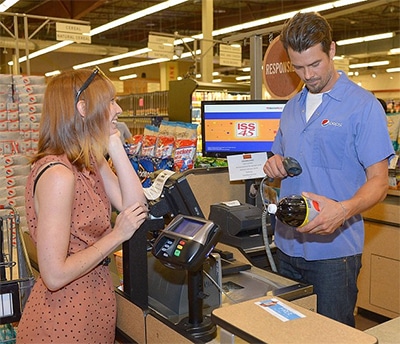
iteration is when you need to do something repeatedly (e.g., ringing in and bagging groceries at the till)

Tidyverse tools for iteration

group_by + summarize: iterate over groups of rows
map_df: iterate over columns

`group_by` + `summarize`

e.g. calculate the average body mass (body_mass_g) for each penguin species from the penguins dataset

In [3]:

#preview data frame
penguins

Out[3]:

To do this we use group_by + summarize to iterate over species, calculating average body mass.

In [5]:

# calculate average body mass for each species

Out[5]:

`summarise()` ungrouping output (override with `.groups` argument)

avg_body_mass <- penguins %>% 
    group_by(species) %>% 
    summarise(avg_body_mass = mean(body_mass_g))
avg_body_mass

What's going on with those NA's?

In [7]:

# calculate average body mass for each species handling NA's

avg_body_mass <- penguins %>% 
    group_by(species) %>% 
    summarise(avg_body_mass = mean(body_mass_g, na.rm = TRUE))
avg_body_mass

`map_df`

e.g. calculate the average rate of each type of crime from the USAarrests data

Be careful: There are a lot of map_... functions that you could use (map, map_lgl, map_chr, etc). Usually in this course we'll only use map_df, but you should investigate the others yourself!

map() is a function for applying a function to each element of a list (similar to lapply() )
map_df() returns a data frame
map() returns a list, map_lgl() a logical vector, map_int() an integer vector, map_dbl() a double vector, and map_chr() a character vector.
map(YOUR_LIST, YOUR_FUNCTION)
This data set contains statistics, in arrests per 100,000 residents for assault, murder, and rape in each of the 50 US states in 1973. Also given is the percent of the population living in urban areas.
Vector, Array, List and Data Frame are 4 basic data types defined in R. Knowing the differences between them will help you use R more efficiently.
Vector: All elements must be of the same type.
Matrix/array: A matrix is a vector with two additional attributes: the number of rows and the number of columns.
List can contain elements of different types.
Dataframe: A data frame is used for storing data tables. It is a list of vectors of equal length.

In [ ]:

head(USArrests)

In [ ]:

#calculate average per capita crime rate for each type of crime

USavg <- map_df(USArrests, mean) # returns a dataframe
USavg

map(USArrests, mean) # returns a list
class(USavg)

Vector, Array, List and Data Frame are 4 basic data types defined in R. Knowing the differences between them will help you use R more efficiently.
Vector: All elements must be of the same type.
Matrix/array: A matrix is a vector with two additional attributes: the number of rows and the number of columns.
List can contain elements of different types.
Dataframe: A data frame is used for storing data tables. It is a list of vectors of equal length.

Go forth and wrangle!

Go to your project groups (different from your breakout rooms)
Work on the group contract (due Jan 30): https://canvas.ubc.ca/courses/59079/assignments/784941
Discuss platforms for working on the group project together (e.g. via Canvas, exchange emails/phone, Slack)
Go ahead and get started on the worksheet! We'll be here to help if you need it.
If any members of your group aren't here today -- reach out to them via Canvas!

image source: https://media.giphy.com/media/Qgm6tIYrSQqC4/giphy-downsized-large.gif

What did we learn?