GitHub Repository: YStrano/DataScience_GA
Path: blob/master/april_18/lessons/lesson-05/code/Jupyter Practice.ipynb
¹⁹⁰⁴ views

Kernel: Python 2

Markdown

In Jupyter notebooks (and on github) we can use Markdown syntax to make nice looking text, include links and images, render code and equations, and organize our presentations.

When you make a new cell in jupyter by either:

Pressing the hotkey combo "shift-enter" to execute a tab
Selecting insert cell from the insert menu

You'll notice that the default cell content-type is "code". To make a cell into a markdown cell, either:

Select "Markdown" from the drop-down menu above, or
Use the hotkey "Ctrl-m" and then press "m"

First exercise

Make this cell into a markdown cell
Run the cell using shift-enter

Hotkeys

There are a ton of useful hotkeys in Jupyter. Pressing "shift-m" puts you into command mode. Pushing another key then usually does something useful. For example,

shift-m then a inserts a new cell above this one
shift-m then b inserts a new cell below

You can find a list of hotkeys here.

Exercise: Practice by making at least one cell above this one and one cell below.

Rendering Code and Equations in Markdown

Enclosing text in backticks will render the text as code. For example, y = a * x + b renders code inline, and three backticks renders code as a block:

def my_function(x):
    return x * x

If you include the language, Jupyter will color the code nicely:

def my_function(x):
    return x * x

If you happen to know about LaTeX, you can also render math equations using two dollar signs $$ like so:

y = a x + b

If the cell already rendered the equation, double-click somewhere in the cell to see the syntax.

Making Links

In Markdown we can link to other sites like so:: [link-name](link-URL), for example: Google. Double-click on the cell to see the synatax.

Exercise:

Insert a new cell below this one
Make a link to General Assembly's webpage
Make a link to our github repository

Embedding Images

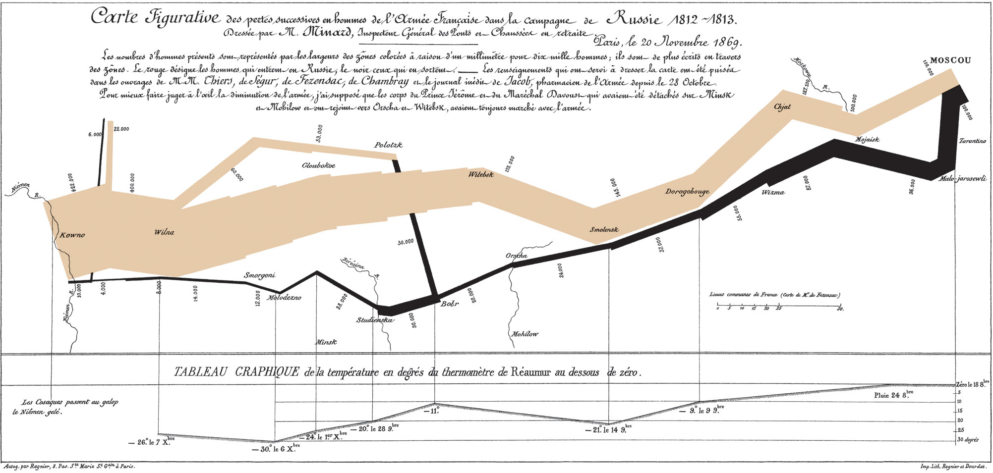
We can also embed images. This is a famous visualization of Napolean's failed invasion of Russia.

Napolean's Invasion

In a new cell, insert an image of your favorite sports team's logo, your favorite animal, or

More Markdown

As data scientists we're often expected to read documentation and apply

Here's a good list of markdown commands. Take a look and then complete the following exercises.

Make three different level headers
Make an ordered list of the data science workflow (seven items!)
Embed the data science workflow image in a new cell (you can find the image on our github page)
Use markdown to make one word in the following sentence bold, one italic, and one strike-through:

The quick brown fox jumps over the lazy dog.

My awesome list

First item
Second item
- sub item

$\alpha$

\int_E {f(e) \, dE}

The quick brown fox jumps over the ~~lazy~~ dog.

Python Practice

Now that we've learned a bit about markdown, try to get into the habit of using markdown to explain and break up your code. This is a good habit because it:

Keeps your code organized
Makes it easier to follow your logic when you present or share
Makes it easier for you to recall your intentions later

Now let's switch gears and practice using Python.

Anything you can do in python you can do in a Jupyter notebook. That includes importing libraries, defining functions, and making plots. Work through the following exercises, and feel free to search for help.

Exercise 1

Print your name using the print command

In [ ]:

Exercise 2

Create a list of the first 10 integers using range

In [4]:

range(11)

Out[4]:

[0, 1, 2, 3, 4, 5, 6, 7, 8, 9, 10]

Exercise 3

Write a function that takes one variable n and sums the squares of the positive numbers less than or equal to n. There are a couple of ways to do this: list comprehensions, a loop, and probably others.

In [5]:

def sum_squares(n):    
    s = 0
    # fill in this part for the sum of squares `s`
    for x in range(n+1):
        s += x * x
#         s += x ** 2
    
    return s

In [28]:

def sum_squares(n):    
    s = 0
    # fill in this part for the sum of squares `s`
    x = 0
    while x < n + 1:        
        s += x * x
        x += 1    
    return s

In [7]:

[x * x for x in range(11)]

Out[7]:

[0, 1, 4, 9, 16, 25, 36, 49, 64, 81, 100]

In [9]:

sum([x * x for x in range(6)])

Out[9]:

55

In [12]:

def sum_squares(n):
    # This function computes the sum of the squares
    # less than and including n 
    s = sum([x * x for x in range(n+1)])    
    return s

In [11]:

sum_squares(5)

Out[11]:

55

Exercise 4

Use your function to find the sum of the first 5 squares.

In [6]:

sum_squares(5)

Out[6]:

55

Exercise 5

It turns out that there is a nice formula for the sum of squares:

\frac{n (n+1) (2n+1)}{6}

Write a new function sum_squares2 that uses this formula. If you used this method above for sum_squares, write the function using a loop instead.

In [13]:

def sum_squares2(n):
    # This function computes the sum of the squares
    # less than and including n 
    s = n * (n + 1) * (2*n + 1) / 6
    return s

In [14]:

sum_squares2(5)

Out[14]:

55

Exercise 6

Compute the sum of the first 20 squares. Do your functions agree?

In [ ]:

Practical Exercises

Hopefully so far so good! Let's learn about some useful libraries now.

Downloading data

We can even download data inside a notebook. This is really useful when you want to scrape websites for data, and for a lot of other purposes like connecting to APIs. Let's try this out using the requests package. If for some reason this isn't installed, you can install it with conda using the graphical interface or from the commandline:

conda install requests

We'll download the famous Boston Housing dataset from the UCI machine learning repository.

In [21]:

# Import the library
import requests

url = "https://archive.ics.uci.edu/ml/machine-learning-databases/housing/housing.data"
# Download the data
r = requests.get(url)
# Save it to disk
with open("housing.csv", "wb") as data:
    data.write(r.content)

Exercise: Try downloading another dataset from the UCI repository (any one you like is fine).

In [20]:

dir(r)
print r.status_code

Out[20]:

200

Now let's open the file with pandas. We'll spend a lot of time getting comfortable with pandas next week. For now let's just load the data into a data frame.

The data doesn't include the column names, so we'll have to add those manually. (Data science isn't always glamorous!) You can find an explanation of the data at the link above.

In [23]:

import pandas as pd
names = ["CRIM", "ZN", "INDUS", "CHAS", "NOX", "RM", "AGE", "DIS", "RAD", "TAX",
           "PTRATIO", "B", "LSTAT", "MEDV"]
data_frame = pd.read_csv("housing.csv", names=names, delim_whitespace=True)

Take a look at the data

In [14]:

data_frame.head()

Out[14]:

Next Steps

If you've made it this far you are doing great! Get a jump start on the next class by poking around with pandas:

Compute the mean and standard deviation of some of the columns. You can get the data like so: data_frame["CRIM"]
Try to make a histogram of some of the columns.
Compute the correlation matrix with data_frame.corr(). Notice anything interesting?
Try to make a scatter plot of some of the strongly correlated columns.

Take a look at the pandas visualization documentation for some ideas on how to make plots.

Try to sketch out a plan of how to use the data science workflow on this dataset. Start by formulating a problem, such as predicting property tax (TAX) from the other variables. What steps have you already completed in the DSW?

In [27]:

import numpy as np

# sum(data_frame["CRIM"]) / len(data_frame["CRIM"])
np.mean(data_frame["CRIM"])

Out[27]:

3.6135235573122535

In [29]:

my_file = open("housing.csv")

In [36]:

with open("housing.csv") as my_file:
    print my_file.readlines()[0]
my_file

Out[36]:

 0.00632  18.00   2.310  0  0.5380  6.5750  65.20  4.0900   1  296.0  15.30 396.90   4.98  24.00

<closed file 'housing.csv', mode 'r' at 0x7fc92c0225d0>

In [37]:

squares = [x*2 for x in range(10)]

In [38]:

squares[3]

Out[38]:

6

In [39]:

data_frame.head()

Out[39]:

In [40]:

data_frame["CRIM"]

Out[40]:

     0.00632
     0.02731
     0.02729
     0.03237
     0.06905
     0.02985
     0.08829
     0.14455
     0.21124
     0.17004
    0.22489
    0.11747
    0.09378
    0.62976
    0.63796
    0.62739
    1.05393
    0.78420
    0.80271
    0.72580
    1.25179
    0.85204
    1.23247
    0.98843
    0.75026
    0.84054
    0.67191
    0.95577
    0.77299
    1.00245
         ...   
   4.87141
  15.02340
  10.23300
  14.33370
   5.82401
   5.70818
   5.73116
   2.81838
   2.37857
   3.67367
   5.69175
   4.83567
   0.15086
   0.18337
   0.20746
   0.10574
   0.11132
   0.17331
   0.27957
   0.17899
   0.28960
   0.26838
   0.23912
   0.17783
   0.22438
   0.06263
   0.04527
   0.06076
   0.10959
   0.04741
Name: CRIM, dtype: float64

In [41]:

my_dict = {"marc": 34, "cecilia": 30}

In [42]:

my_dict[0]

Out[42]:

---------------------------------------------------------------------------
KeyError                                  Traceback (most recent call last)
<ipython-input-42-085e2dd1e3fc> in <module>()
----> 1 my_dict[0]

KeyError: 0

In [43]:

my_dict["marc"]

Out[43]:

34

In [1]:

import matplotlib.pyplot as plt

plt.scatter(range(0, 10), [x*x for x in range(0, 10)])

Out[1]:

<matplotlib.collections.PathCollection at 0x7fc46a4cb5d0>

In [2]:

plt.show()

In [ ]: