Lesson 5 - Data structures.ipynb

Kernel: Python 3 (ipykernel)

Lesson 5 - Data structures

Authors:

• Yilber Fabian Bautista

• Sean Tulin

For numerical calculations, it is important to consider how numerical data will be organized. We already learned about lists and arrays, which are examples of data structures and are useful for organizing numerical values.

Here we introduce new types of data structures. First, we introduce dictionaries, which are built-in to Python. Second, we introduce the pandas library, which the most widely-used Python library for data analysis.

Objectives:

• Learn how to use Python dictionaries

• Gain familiarity and perform basic tasks with the pandas library:

  • Learn how to use DataFrames

  • Learn how to create, modify, save, and read data files in csv (comma separated values) format

  • Plot data using pandas library

Dictionaries

A dictionary consists of keys and values assigned to those keys, often referred to as key-value pairs. Since dictionaries have similar characteristics to lists, it is helpful to compare these two

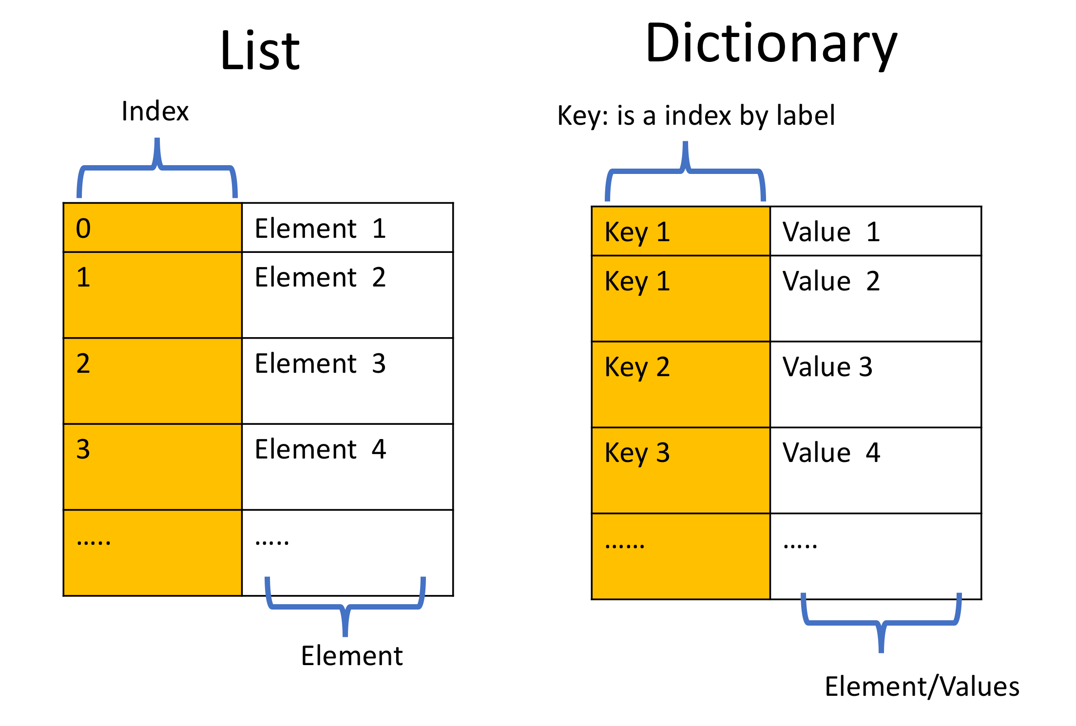
Figure taken from IBM courses

Instead of the numerical indices, dictionaries are indexed by keys. Keys are typically strings, but any non-mutable objects (like tuples) can also serve as a key. Keys play the role of indices used to access values within a dictionary.

Similar to lists, dictionaries are mutable objects, which means we can modify them, change values for a given key, add new key-value pairs, etc.

The python syntax to create a dictionary is as follows. Here is a simple dictionary with one key-value pair.

my_dictionary = {'key':value}

Larger dictionaries are created by separating each key-value pair with a comma, e.g.,

my_dictionary = {'key1':value1, 'key2':value2}

The type of a dictionary is dict.

Let's create our first dictionary in python below. Note we illustrate:

• Keys need not all be the same type. Typically, all keys will be strings, but other types can be keys too.

• Values also need not be the same type, similar to lists and tuples.

import numpy as np

# Create the dictionary

my_dictionary = {"key1": 1, "key2": "2", "key3": np.array([3, 3, 8]),
                 "key4": (4, 4, '4'), ('key5'): 5, (0, 1): 6}

type(my_dictionary)

dict

Accessing the keys of a dictionary:

Every dictionary has a built-in method keys() to obtain a list of the keys of the dictionary (if you do not know them ahead of time).

my_dictionary.keys()

Accessing the value by the key:

To access the value for given key, we have two options:

• Using square brackets similar to accessing elements of a list:

my_dictionary['key1']

• Using the built-in method get():

my_dictionary.get('key1')

Both options will return the output 1. However, they behave differently if a key is not in the dictionary. For example, my_dictionary['key7'] will produce an error message, while my_dictionary.get('key7') will yield None (with no error message). You can use a syntax like

if my_dictionary.get('key'):
    <Do something>

to perform an action only if 'key' is found in the dictionary.

Adding new key-value pairs to the dictionary

For lists and arrays we would had use the list.append(value) and np.append(array,value) methods respectively. For dictionaries instead, we will use the following syntax:

my_dictionary['key7'] = 'new_value'

Remove a key-value pair from a dictionary

To remove a key-value pair, we use the pop() method. For instance,

value = my_dictionary.pop('key7')

will set value equal to 'new_value' and it will delete this key-value pair from our dictionary. Now if we ask for the keys of our dictionary

my_dictionary.keys()

we will get as output dict_keys(['key1', 'key2', 'key3', 'key4', 'key5', (0, 1)]). If we wanted to delete this key-value pair without retaining the value, we can simply do

my_dictionary.pop('key7')

without assigning it to a variable.

See this link for additional methods applied to dictionaries

Exercise 1

1. Type out all the commands yourself for the previous lines of code.

2. Given the following dictionaries, write short line codes to answer the following questions (See this page for more exercises with dictionaries):

dictionary_1 ={"name": "Plato", "country": "Ancient Greece", "born": -427, "teacher": "Socrates", "student": "Aristotle"}
dictionary_2 = {"son's name": "Lucas", "son's eyes": "green", "son's height": 32, "son's weight": 25}

• When was Plato born?

• Change Plato's birth year from B.C. 427 to B.C. 428.

• Add the key "work" to dictionary_1, with the values "Apology", "Phaedo", "Republic", "Symposium" in a list.

• Add 2 inches to the son's height in dictionary_2.

• Using the .get() method, print the value of "son's eyes".

• Merge dictionary_1 and dictionary_2 into the dictionary dictionary_merge, using the syntax:

dictionary_merge = merge(**dictionary_1,**dictionary_2)

and print the list of keys in dictionary_merge.

The pandas library

The pandas library is used to efficiently manipulate tabular data such as data stored in spreadsheets or databases, and to do statistics analysis of such data. Pandas supports the integration of several file formats and data sources. Here we focus on csv files, but many others are supported as well (e.g., excel, sql, json).

You import it as follows:

import pandas as pd

For a detail view of pandas library, see here, and for Library Highlights see here.

In pandas, DataFrame objects are the key data structures that are used to store your data. You can think of a DataFrame as a spreadsheet.

Let us start our pandas journey by creating simple DataFrames from the data structure we learned above, namely, dictionaries. We create a DataFrame from a dictionary of lists. Then, the dictionary keys will be used as column headers and the values in each list will be the columns.

import pandas as pd

# Create a dictionary

dictionary =  {"Name": ["Braund, Mr. Owen Harris","Allen, Mr. William Henry","Bonnell, Ms. Elizabeth"],
               "Age": [22, 35, 25],
               "Course": ["Data Structures", "Machine Learning", "OOPS with java"]}

# Now create a DataFrame from a dictionary

df = pd.DataFrame(dictionary)

# Print out the DataFrame
df

Exercise 2

Get some experience with DataFrames by creating your own DataFrame, similar to the one defined above. (Avoid coping and pasting the code from the text.)

Working with DataFrames

DataFrames have many built-in methods and attributes that make them easy to work with. Here we go through the basics.

The head/tail attributes

The built-in methods head(i) and tail(i) access the first or last i elements of your DataFrame, e.g., df.head(2) will access the first two elements. This is useful when dealing with large datasets.

Slicing a DataFrame

To access a desired slice of a DataFrame, we use a similar syntax that for lists. For example

sub_df = df[1:3]

takes the slice containing the second and third elements of df and saves them in the new DataFrame named sub_df, with the same attributes as the original DataFrame df.

Keys in a DataFrame

As for dictionaries, we can ask for the keys of a DataFrame using the keys() method. In our df example

df.keys()

we get as output Index(['Name', 'Age', 'Course'], dtype='object').

One can also access the keys using the attribute columns.

df.columns

Accessing a column in a DataFrame

Columns in the DataFrame are labeled by keys, using the same syntax as for dictionaries. For instance, to access the column containing all of the names in our df defined above we use:

df['Name']

Note that this produces as an output a list-like pandas.Series object with all elements of the 'Name' column. You can convert this to a true list using

list(df['Name'])

Accessing a row in a DataFrame

To access row j in our DataFrame, we use the attribute iloc[j]. For example

Allen_info = df.iloc[1]

will save the 2nd row of df as Allen_info. If we print(Allen_info), we have the following key-value pairs

Name      Allen, Mr. William Henry
Age                             35
Course            Machine Learning
Name: 1, dtype: object

Allen_info behaves like a dictionary, for example, Allen_info['Age'] will return 35.

Accessing a single element in a DataFrame

According to our previous discussion, there are two options to access a single element of a DataFrame. For example, suppose we want Allen's age:

• Taking the 'Age' entry of the Allen row, as above: df.iloc[1]['Age']

• Taking the 2nd entry of the 'Age' column: df['Age'][1]

with both methods producing the output 35.

# Try this out yourself in this cell

Adding a new row to the DataFrame

Similar to lists, each DataFrame has a built-in method append() that can add a new row. Since the DataFrame has several entries, we need first to create a dictionary, which will be added to the DataFrame. Let us see how this work with the following example.

sara_info = {'Name':'Sara Remmen', 'Age': 20, 'Course':'Python programing','Grade': 10}

# Adding the new dictionary
df2 = df.append(sara_info, ignore_index=True)
df2

There are a few things to mention:

• We have added a new key 'Grade' to the dictionary, which creates a new column in the DataFrame. Since previous entries do not have values for this key, they are set to NaN for the other rows.

• Unlike lists, using append() does not modify the original DataFrame df. If we want to save the modified DataFrame, we need to assign df.append() to something, e.g., df2.

If we want to modify df directly, we can use the loc[i] attribute, where i is the position we want to add the new row. Here is an example. (Note in this case, the new row must have the same number of entries as the existing DataFrame rows.)

df.loc[3] = ['Nathan S.', 20, 'Julia programing']
df

Changing an entry in your DataFrame

You can use loc[row,col] to change entries in your DataFrame, labeled by row row and column col. Here is an example where we change Allen's Grade from NaN to 8.

df2.loc[2,'Grade'] = 8 
df2

Removing a whole row in a DataFrame

To delete a row, we use the built-in method drop. For instance, let us remove the entry for Sara's info from df2, which is labeled as row 3. The syntax is

df3 = df2.drop(labels=3)

Note that by default drop() does not modify the original DataFrame, so we have assigned it to a new DataFrame df3. If we want to modify the original DataFrame, we set the keyword inplace=True, as follows:

df2.drop(labels=3,inplace=True)

However, be careful when using this option since once rows are removed, we cannot recover them.

# Some space to write your own code

Adding a new column to the DataFrame

To add a complete column, we use a syntax similar to dictionaries. We have to specify all the elements of the column in a list, whose length has to match the length of the DataFrame. In our previous examples we would have made.

df2['Major'] =  ['Physics and Astronomy', 'Computer Science', 'Physics and Astronomy', 'Maths']

#some space for coding

Merging two (or more) DataFrames

One of the main advantages of pandas is that it offers high performance merging and joining of data sets with the same number of columns. Let's see it in an specific example. (Note that the ignore_index=True keyword is needed to ignore previous row labels and relabel the indices of the rows in the merged DataFrame, whereas sort=True keyword will display the DataFrame in an ordered form depending on the order of the two entries)

merged_df = pd.concat([df,df2],ignore_index=True,sort=True)
merged_df

Loading and saving DataFrames

A csv file, which stands for Comma Separated Values, is a useful format for storing small-to-medium-sized data sets in plain text format. First, we consider loading a file and saving it to a DataFrame. The syntax for Mac and Linux is

df = pd.read_csv("directory1/directory2/file_name.csv")

and for Windows the syntax is

df = pd.read_csv("directory1\\directory2\\file_name.csv")

That is, the separator between directory names is / for Mac and Linux, and \\ for Windows.

Similarly, the syntax for saving a DataFrame is:

df.to_csv('directory1/directory2/file_name.csv',index=False)

whereas for Windows the syntax is

df.to_csv('directory1\\directory2\\file_name.csv',index=False)

If the entire path of directories is not specified, the file will be loaded or saved in the same folder of our jupyter notebook. The keyword index=False is useful, otherwise the row index is also saved in the csv file too.

Plotting data from DataFrames

DataFrames have a built-in method plot() for quickly plotting the data they contain data. For more on plotting see the Chart Visualization.

Here is an example for loading, plotting, and saving some data.

# First, load the data and get a quick view of what it contains

df = pd.read_csv('saving_example.csv')
df.head(5)

# Next, make a plot

df.plot('x','y',kind='scatter')

# Create a new column
# Define new variable w = x*y

df['w'] = df['x']*df['y']

df.plot('x','w',kind='scatter')

# Save the new DataFrame
# Using the same name will overwrite the original file

df.to_csv('saving_example.csv',index=False)

Exercise 3

Galaxy rotation curve

The Directory Rotation curves, contains data sets for the rotation curve for several Dwarf galaxies. See rotation curves for a detail description of the data files. In this exercise we will practice our pandas skills on those files (They will also be used in Tutorial 6 using classes, and in Tutorial 7, when we discuss interpolating function). By the end of this exercise we will obtain our Dark Matter rotation curve $$v_{DM}(r) = \sqrt{v_c^2(r)-v_{star}^2(r)-v_{gas}^2(r)} \, ,$$ as well as our DM mass distribution $$M_{DM}(r) = r v^2_{DM}(r)/G_N \, .$$

We will take distance $r$ to be in units of kiloparsecs, velocity $v$ to be in units of $km/s$, and mass $M$ in solar masses $M_\odot$. Hence, it is useful to take Newton's gravitational constant in these units as $G_N = 4.302 \times 10^{-6} km^2/s^2\times kpc/M_{sol}$.

Let us divide the exercise in several steps:

1. Choose your favorite galaxy in the Rotation curves directory, i.e. identify the two files RotationCurve galaxy.csv and RotationCurve baryons galaxy.csv.

2. Create the DataFrame df_circular for the chosen galaxy, which will load the data contained in the file RotationCurve galaxy.csv. It should look similar to the following example for Galaxy 'IC2574':

3. Add a new column to df_circular that contains the DM mass. For simplicity we will assume $v_{star}=v_{gas} = 0$, and therefore $v_{DM}(r)=v_c(r)$ . We will return to this simplification in Tutorial 7.

4. Make a plot of $M_{DM}(r)$ as function of $r$, using pandas plotting tools.

5. Save the data including the new column into a new csv file.

Exercise 4 (Optional)

In this exercise we will plot the DM velocity having into account errors in the measurements as well as systematic errors.

1. As explained in rotation curves, some of the measured errors (i.e. some values in circ velocity error) have been underestimated. In this step we will include a systematic error at the level of 5% of the last measured velocity point (i.e. the last data point of column cir velocity in our df_circular). Add a new column in df_circular called syst error whose values contain the systematic error. Then, add the new column total error, containing the total error computed as the sum in quadratures of sys error and circ velocity error.

2. Using matplotlib.pyplot.errorbar library, do an errorbar plot of the circular velocity as a function of radial distance, where the errorbars are given by total error in df_circular.

3. Save the data including the new error columns into a new csv file