8.4-generating-images-with-vaes.ipynb

Kernel: Python 3

import keras
keras.__version__

'2.0.8'

from keras import backend as K
K.clear_session()

Generating images

This notebook contains the second code sample found in Chapter 8, Section 4 of Deep Learning with Python. Note that the original text features far more content, in particular further explanations and figures: in this notebook, you will only find source code and related comments.

---

Variational autoencoders

Variational autoencoders, simultaneously discovered by Kingma & Welling in December 2013, and Rezende, Mohamed & Wierstra in January 2014, are a kind of generative model that is especially appropriate for the task of image editing via concept vectors. They are a modern take on autoencoders -- a type of network that aims to "encode" an input to a low-dimensional latent space then "decode" it back -- that mixes ideas from deep learning with Bayesian inference.

A classical image autoencoder takes an image, maps it to a latent vector space via an "encoder" module, then decode it back to an output with the same dimensions as the original image, via a "decoder" module. It is then trained by using as target data the same images as the input images, meaning that the autoencoder learns to reconstruct the original inputs. By imposing various constraints on the "code", i.e. the output of the encoder, one can get the autoencoder to learn more or less interesting latent representations of the data. Most commonly, one would constraint the code to be very low-dimensional and sparse (i.e. mostly zeros), in which case the encoder acts as a way to compress the input data into fewer bits of information.

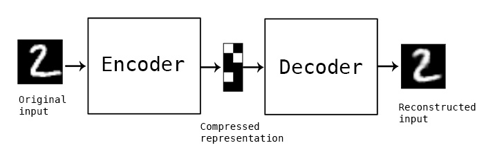
In practice, such classical autoencoders don't lead to particularly useful or well-structured latent spaces. They're not particularly good at compression, either. For these reasons, they have largely fallen out of fashion over the past years. Variational autoencoders, however, augment autoencoders with a little bit of statistical magic that forces them to learn continuous, highly structured latent spaces. They have turned out to be a very powerful tool for image generation.

A VAE, instead of compressing its input image into a fixed "code" in the latent space, turns the image into the parameters of a statistical distribution: a mean and a variance. Essentially, this means that we are assuming that the input image has been generated by a statistical process, and that the randomness of this process should be taken into accounting during encoding and decoding. The VAE then uses the mean and variance parameters to randomly sample one element of the distribution, and decodes that element back to the original input. The stochasticity of this process improves robustness and forces the latent space to encode meaningful representations everywhere, i.e. every point sampled in the latent will be decoded to a valid output.

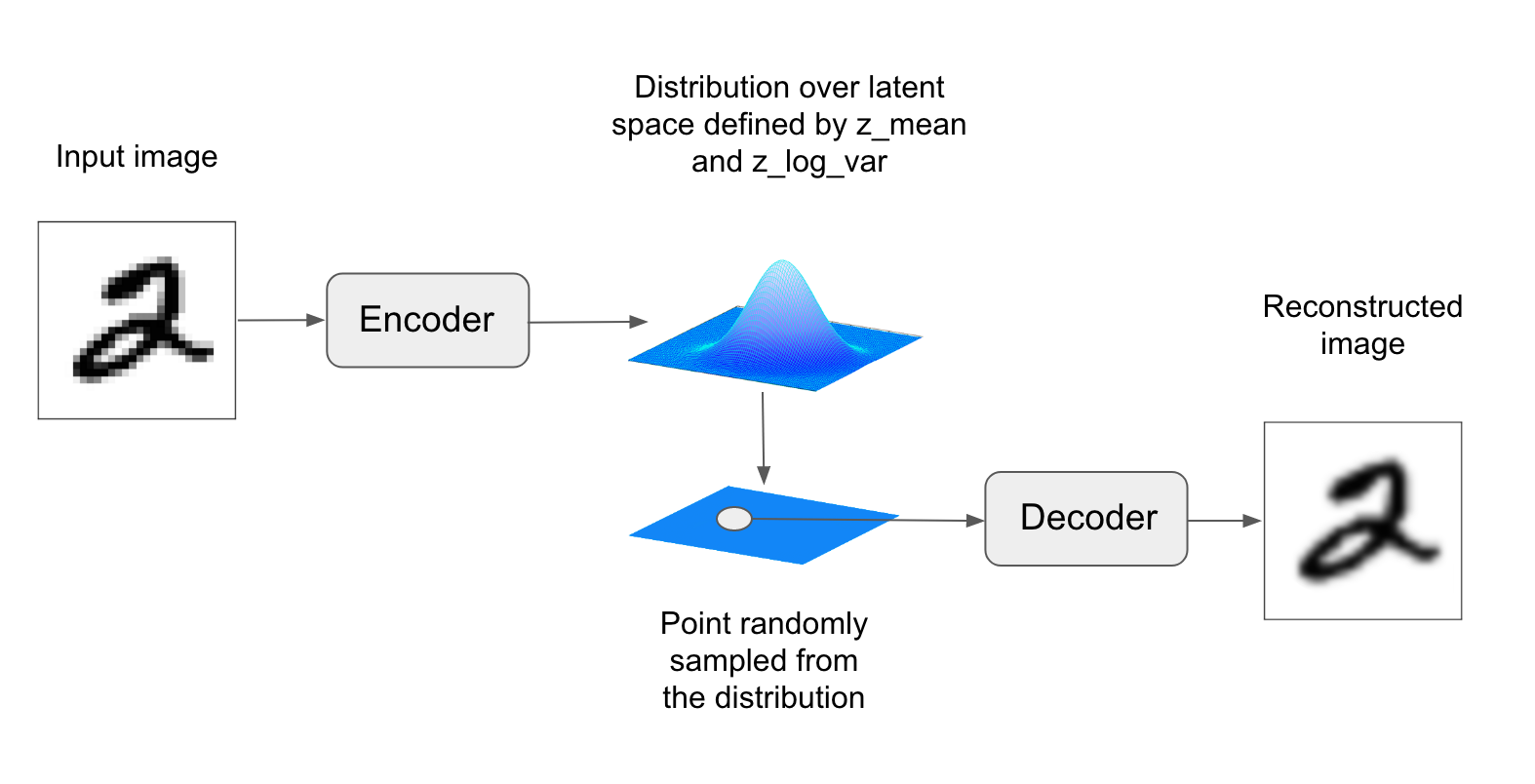
In technical terms, here is how a variational autoencoder works. First, an encoder module turns the input samples input_img into two parameters in a latent space of representations, which we will note z_mean and z_log_variance. Then, we randomly sample a point z from the latent normal distribution that is assumed to generate the input image, via z = z_mean + exp(z_log_variance) * epsilon, where epsilon is a random tensor of small values. Finally, a decoder module will map this point in the latent space back to the original input image. Because epsilon is random, the process ensures that every point that is close to the latent location where we encoded input_img (z-mean) can be decoded to something similar to input_img, thus forcing the latent space to be continuously meaningful. Any two close points in the latent space will decode to highly similar images. Continuity, combined with the low dimensionality of the latent space, forces every direction in the latent space to encode a meaningful axis of variation of the data, making the latent space very structured and thus highly suitable to manipulation via concept vectors.

The parameters of a VAE are trained via two loss functions: first, a reconstruction loss that forces the decoded samples to match the initial inputs, and a regularization loss, which helps in learning well-formed latent spaces and reducing overfitting to the training data.

Let's quickly go over a Keras implementation of a VAE. Schematically, it looks like this:

# Encode the input into a mean and variance parameter
z_mean, z_log_variance = encoder(input_img)

# Draw a latent point using a small random epsilon
z = z_mean + exp(z_log_variance) * epsilon

# Then decode z back to an image
reconstructed_img = decoder(z)

# Instantiate a model
model = Model(input_img, reconstructed_img)

# Then train the model using 2 losses:
# a reconstruction loss and a regularization loss

Here is the encoder network we will use: a very simple convnet which maps the input image x to two vectors, z_mean and z_log_variance.

import keras
from keras import layers
from keras import backend as K
from keras.models import Model
import numpy as np

img_shape = (28, 28, 1)
batch_size = 16
latent_dim = 2  # Dimensionality of the latent space: a plane

input_img = keras.Input(shape=img_shape)

x = layers.Conv2D(32, 3,
                  padding='same', activation='relu')(input_img)
x = layers.Conv2D(64, 3,
                  padding='same', activation='relu',
                  strides=(2, 2))(x)
x = layers.Conv2D(64, 3,
                  padding='same', activation='relu')(x)
x = layers.Conv2D(64, 3,
                  padding='same', activation='relu')(x)
shape_before_flattening = K.int_shape(x)

x = layers.Flatten()(x)
x = layers.Dense(32, activation='relu')(x)

z_mean = layers.Dense(latent_dim)(x)
z_log_var = layers.Dense(latent_dim)(x)

Here is the code for using z_mean and z_log_var, the parameters of the statistical distribution assumed to have produced input_img, to generate a latent space point z. Here, we wrap some arbitrary code (built on top of Keras backend primitives) into a Lambda layer. In Keras, everything needs to be a layer, so code that isn't part of a built-in layer should be wrapped in a Lambda (or else, in a custom layer).

def sampling(args):
    z_mean, z_log_var = args
    epsilon = K.random_normal(shape=(K.shape(z_mean)[0], latent_dim),
                              mean=0., stddev=1.)
    return z_mean + K.exp(z_log_var) * epsilon

z = layers.Lambda(sampling)([z_mean, z_log_var])

This is the decoder implementation: we reshape the vector z to the dimensions of an image, then we use a few convolution layers to obtain a final image output that has the same dimensions as the original input_img.

# This is the input where we will feed `z`.
decoder_input = layers.Input(K.int_shape(z)[1:])

# Upsample to the correct number of units
x = layers.Dense(np.prod(shape_before_flattening[1:]),
                 activation='relu')(decoder_input)

# Reshape into an image of the same shape as before our last `Flatten` layer
x = layers.Reshape(shape_before_flattening[1:])(x)

# We then apply then reverse operation to the initial
# stack of convolution layers: a `Conv2DTranspose` layers
# with corresponding parameters.
x = layers.Conv2DTranspose(32, 3,
                           padding='same', activation='relu',
                           strides=(2, 2))(x)
x = layers.Conv2D(1, 3,
                  padding='same', activation='sigmoid')(x)
# We end up with a feature map of the same size as the original input.

# This is our decoder model.
decoder = Model(decoder_input, x)

# We then apply it to `z` to recover the decoded `z`.
z_decoded = decoder(z)

The dual loss of a VAE doesn't fit the traditional expectation of a sample-wise function of the form loss(input, target). Thus, we set up the loss by writing a custom layer with internally leverages the built-in add_loss layer method to create an arbitrary loss.

class CustomVariationalLayer(keras.layers.Layer):

    def vae_loss(self, x, z_decoded):
        x = K.flatten(x)
        z_decoded = K.flatten(z_decoded)
        xent_loss = keras.metrics.binary_crossentropy(x, z_decoded)
        kl_loss = -5e-4 * K.mean(
            1 + z_log_var - K.square(z_mean) - K.exp(z_log_var), axis=-1)
        return K.mean(xent_loss + kl_loss)

    def call(self, inputs):
        x = inputs[0]
        z_decoded = inputs[1]
        loss = self.vae_loss(x, z_decoded)
        self.add_loss(loss, inputs=inputs)
        # We don't use this output.
        return x

# We call our custom layer on the input and the decoded output,
# to obtain the final model output.
y = CustomVariationalLayer()([input_img, z_decoded])

Finally, we instantiate and train the model. Since the loss has been taken care of in our custom layer, we don't specify an external loss at compile time (loss=None), which in turns means that we won't pass target data during training (as you can see we only pass x_train to the model in fit).

from keras.datasets import mnist

vae = Model(input_img, y)
vae.compile(optimizer='rmsprop', loss=None)
vae.summary()

# Train the VAE on MNIST digits
(x_train, _), (x_test, y_test) = mnist.load_data()

x_train = x_train.astype('float32') / 255.
x_train = x_train.reshape(x_train.shape + (1,))
x_test = x_test.astype('float32') / 255.
x_test = x_test.reshape(x_test.shape + (1,))

vae.fit(x=x_train, y=None,
        shuffle=True,
        epochs=10,
        batch_size=batch_size,
        validation_data=(x_test, None))

/usr/local/lib/python3.5/dist-packages/ipykernel_launcher.py:4: UserWarning: Output "custom_variational_layer_1" missing from loss dictionary. We assume this was done on purpose, and we will not be expecting any data to be passed to "custom_variational_layer_1" during training.
  after removing the cwd from sys.path.

____________________________________________________________________________________________________
Layer (type)                     Output Shape          Param #     Connected to                     
====================================================================================================
input_1 (InputLayer)             (None, 28, 28, 1)     0                                            
____________________________________________________________________________________________________
conv2d_1 (Conv2D)                (None, 28, 28, 32)    320         input_1[0][0]                    
____________________________________________________________________________________________________
conv2d_2 (Conv2D)                (None, 14, 14, 64)    18496       conv2d_1[0][0]                   
____________________________________________________________________________________________________
conv2d_3 (Conv2D)                (None, 14, 14, 64)    36928       conv2d_2[0][0]                   
____________________________________________________________________________________________________
conv2d_4 (Conv2D)                (None, 14, 14, 64)    36928       conv2d_3[0][0]                   
____________________________________________________________________________________________________
flatten_1 (Flatten)              (None, 12544)         0           conv2d_4[0][0]                   
____________________________________________________________________________________________________
dense_1 (Dense)                  (None, 32)            401440      flatten_1[0][0]                  
____________________________________________________________________________________________________
dense_2 (Dense)                  (None, 2)             66          dense_1[0][0]                    
____________________________________________________________________________________________________
dense_3 (Dense)                  (None, 2)             66          dense_1[0][0]                    
____________________________________________________________________________________________________
lambda_1 (Lambda)                (None, 2)             0           dense_2[0][0]                    
                                                                   dense_3[0][0]                    
____________________________________________________________________________________________________
model_1 (Model)                  (None, 28, 28, 1)     56385       lambda_1[0][0]                   
____________________________________________________________________________________________________
custom_variational_layer_1 (Cust [(None, 28, 28, 1), ( 0           input_1[0][0]                    
                                                                   model_1[1][0]                    
====================================================================================================
Total params: 550,629
Trainable params: 550,629
Non-trainable params: 0
____________________________________________________________________________________________________
Train on 60000 samples, validate on 10000 samples
Epoch 1/10
60000/60000 [==============================] - 52s - loss: 0.2109 - val_loss: 0.1966
Epoch 2/10
60000/60000 [==============================] - 51s - loss: 0.1933 - val_loss: 0.1899
Epoch 3/10
60000/60000 [==============================] - 51s - loss: 0.1886 - val_loss: 0.1862
Epoch 4/10
60000/60000 [==============================] - 51s - loss: 0.1858 - val_loss: 0.1851
Epoch 5/10
60000/60000 [==============================] - 51s - loss: 0.1840 - val_loss: 0.1830
Epoch 6/10
60000/60000 [==============================] - 51s - loss: 0.1827 - val_loss: 0.1816
Epoch 7/10
60000/60000 [==============================] - 51s - loss: 0.1816 - val_loss: 0.1813
Epoch 8/10
60000/60000 [==============================] - 51s - loss: 0.1807 - val_loss: 0.1827
Epoch 9/10
60000/60000 [==============================] - 51s - loss: 0.1800 - val_loss: 0.1806
Epoch 10/10
60000/60000 [==============================] - 51s - loss: 0.1794 - val_loss: 0.1801

<keras.callbacks.History at 0x7fe9b9870470>

Once such a model is trained -- e.g. on MNIST, in our case -- we can use the decoder network to turn arbitrary latent space vectors into images:

import matplotlib.pyplot as plt
from scipy.stats import norm

# Display a 2D manifold of the digits
n = 15  # figure with 15x15 digits
digit_size = 28
figure = np.zeros((digit_size * n, digit_size * n))
# Linearly spaced coordinates on the unit square were transformed
# through the inverse CDF (ppf) of the Gaussian
# to produce values of the latent variables z,
# since the prior of the latent space is Gaussian
grid_x = norm.ppf(np.linspace(0.05, 0.95, n))
grid_y = norm.ppf(np.linspace(0.05, 0.95, n))

for i, yi in enumerate(grid_x):
    for j, xi in enumerate(grid_y):
        z_sample = np.array([[xi, yi]])
        z_sample = np.tile(z_sample, batch_size).reshape(batch_size, 2)
        x_decoded = decoder.predict(z_sample, batch_size=batch_size)
        digit = x_decoded[0].reshape(digit_size, digit_size)
        figure[i * digit_size: (i + 1) * digit_size,
               j * digit_size: (j + 1) * digit_size] = digit

plt.figure(figsize=(10, 10))
plt.imshow(figure, cmap='Greys_r')
plt.show()

The grid of sampled digits shows a completely continuous distribution of the different digit classes, with one digit morphing into another as you follow a path through latent space. Specific directions in this space have a meaning, e.g. there is a direction for "four-ness", "one-ness", etc.