12_object_based_methods.ipynb

Kernel: Python 3

View source on GitHub

Notebook Viewer

Run in Google Colab

Object-based methods

Image objects are sets of connected pixels having the same integer value. Categorical, binned, and boolean image data are suitable for object analysis.

Earth Engine offers methods for labeling each object with a unique ID, counting the number of pixels composing objects, and computing statistics for values of pixels that intersect objects.

• connectedComponents(): label each object with a unique identifier.

• connectedPixelCount(): compute the number of pixels in each object.

• reduceConnectedComponents(): compute a statistic for pixels in each object.

Caution: results of object-based methods depend on scale, which is determined by:

• the requested scale of an output (e.g., Export.image.toAsset() or Export.image.toDrive()).

• functions that require a scale of analysis (e.g., reduceRegions() or reduceToVectors()).

• Map zoom level. Take special note of scale determined by Map zoom level. Results of object-based methods will vary when viewing or inspecting image layers in the Map, as each pyramid layer has a different scale. To force a desired scale of analysis in Map exploration, use reproject(). However, it is strongly recommended that you NOT use reproject() because the entire area visible in the Map will be requested at the set scale and projection. At large extents this can cause too much data to be requested, often triggering errors. Within the image pyramid-based architecture of Earth Engine, scale and projection need only be set for operations that provide scale and crs as parameters. See Scale of Analysis and Reprojecting for more information.

Install Earth Engine API and geemap

Install the Earth Engine Python API and geemap. The geemap Python package is built upon the ipyleaflet and folium packages and implements several methods for interacting with Earth Engine data layers, such as Map.addLayer(), Map.setCenter(), and Map.centerObject(). The following script checks if the geemap package has been installed. If not, it will install geemap, which automatically installs its dependencies, including earthengine-api, folium, and ipyleaflet.

Important note: A key difference between folium and ipyleaflet is that ipyleaflet is built upon ipywidgets and allows bidirectional communication between the front-end and the backend enabling the use of the map to capture user input, while folium is meant for displaying static data only (source). Note that Google Colab currently does not support ipyleaflet (source). Therefore, if you are using geemap with Google Colab, you should use import geemap.foliumap. If you are using geemap with binder or a local Jupyter notebook server, you can use import geemap, which provides more functionalities for capturing user input (e.g., mouse-clicking and moving).

# Installs geemap package
import subprocess

try:
    import geemap
except ImportError:
    print("geemap package not installed. Installing ...")
    subprocess.check_call(["python", "-m", "pip", "install", "geemap"])

# Checks whether this notebook is running on Google Colab
try:
    import google.colab
    import geemap.foliumap as emap
except:
    import geemap as emap

# Authenticates and initializes Earth Engine
import ee

try:
    ee.Initialize()
except Exception as e:
    ee.Authenticate()
    ee.Initialize()

Create an interactive map

The default basemap is Google Satellite. Additional basemaps can be added using the Map.add_basemap() function.

Map = geemap.Map(center=[40, -100], zoom=4)
Map.add_basemap("ROADMAP")  # Add Google Map
Map

Add Earth Engine Python script

Example setup

The following sections provide examples of object-based methods applied to Landsat 8 surface temperature with each section building on the former. Run the next snippet to generate the base image: thermal hotspots (> 303 degrees Kelvin) for a small region of San Francisco (Figure 1).

# Make an area of interest geometry centered on San Francisco.
point = ee.Geometry.Point(-122.1899, 37.5010)
aoi = point.buffer(10000)

# Import a Landsat 8 image, subset the thermal band, and clip to the
# area of interest.
kelvin = (
    ee.Image("LANDSAT/LC08/C01/T1_TOA/LC08_044034_20140318")
    .select(["B10"], ["kelvin"])
    .clip(aoi)
)

# Display the thermal band.
# Map.centerObject(point, 13)
Map.setCenter(-122.1899, 37.5010, 13)
Map.addLayer(kelvin, {"min": 288, "max": 305}, "Kelvin")


# Threshold the thermal band to set hot pixels as value 1 and not as 0.
hotspots = kelvin.gt(303).selfMask().rename("hotspots")

# Display the thermal hotspots on the Map.
Map.addLayer(hotspots, {"palette": "FF0000"}, "Hotspots")

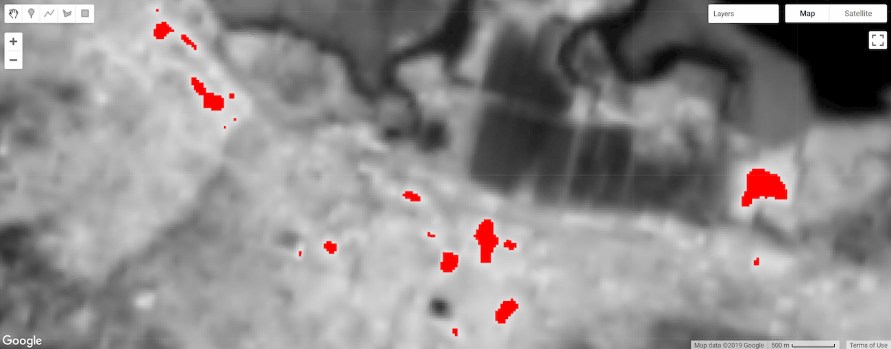
Figure 1. Temperature for a region of San Francisco. Pixels with temperature greater than 303 degrees Kelvin are distinguished by the color red (thermal hotspots).

Label objects

Labeling objects is often the first step in object analysis. Here, the connectedComponents() function is used to identify image objects and assign a unique ID to each; all pixels belonging to an object are assigned the same integer ID value. The result is a copy of the input image with an additional "labels" band associating pixels with an object ID value based on connectivity of pixels in the first band of the image (Figure 2).

# Uniquely label the hotspot image objects.
objectId = hotspots.connectedComponents(
    **{"connectedness": ee.Kernel.plus(1), "maxSize": 128}
)

# Display the uniquely ID'ed objects to the Map.
Map.addLayer(objectId.randomVisualizer(), {}, "Objects")

Note that the maximum patch size is set to 128 pixels; objects composed of more pixels are masked. The connectivity is specified by an ee.Kernel.plus(1) kernel, which defines four-neighbor connectivity; use ee.Kernel.square(1) for eight-neighbor.

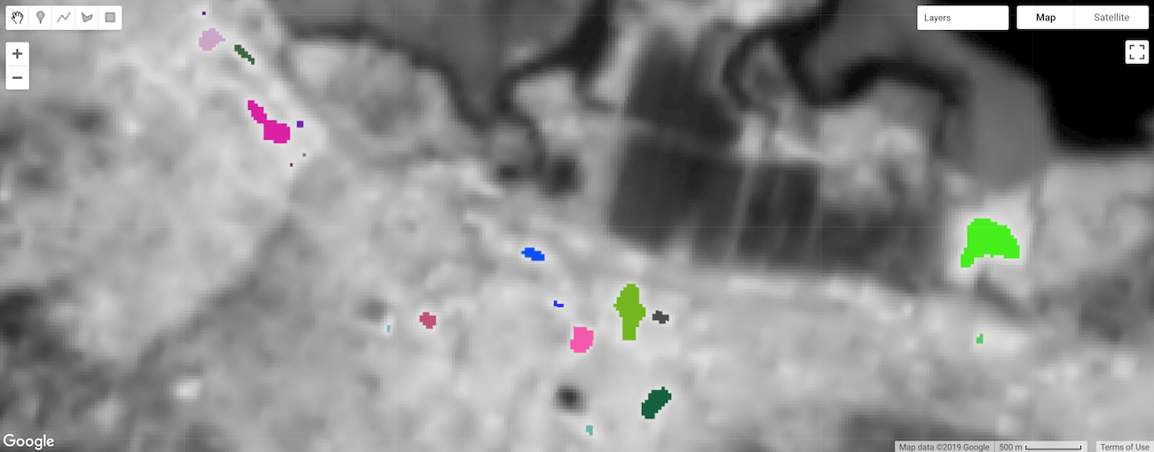
Figure 2. Thermal hotspot objects labeled and styled by a unique ID.

Object size

Number of pixels Calculate the number of pixels composing objects using the connectedPixelCount() image method. Knowing the number of pixels in an object can be helpful for masking objects by size and calculating object area. The following snippet applies connectedPixelCount() to the "labels" band of the objectId image defined in the previous section.

# Compute the number of pixels in each object defined by the "labels" band.
objectSize = objectId.select("labels").connectedPixelCount(
    **{"maxSize": 128, "eightConnected": False}
)

# Display object pixel count to the Map.
Map.addLayer(objectSize, {}, "Object n pixels")

connectedPixelCount() returns a copy of the input image where each pixel of each band contains the number of connected neighbors according to either the four- or eight-neighbor connectivity rule determined by a boolean argument passed to the eightConnected parameter. Note that connectivity is determined independently for each band of the input image. In this example, a single-band image (objectId) representing object ID was provided as input, so a single-band image was returned with a "labels" band (present as such in the input image), but now the values represent the number of pixels composing objects; every pixel of each object will have the same pixel count value (Figure 3).

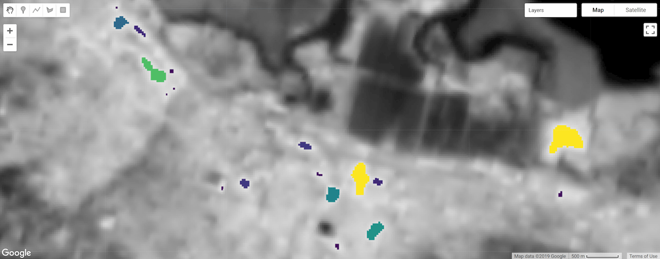
Figure 3. Thermal hotspot objects labeled and styled by size.

Area

Calculate object area by multiplying the area of a single pixel by the number of pixels composing an object (determined by connectedPixelCount()). Pixel area is provided by an image generated from ee.Image.pixelArea().

# Get a pixel area image.
pixelArea = ee.Image.pixelArea()

# Multiply pixel area by the number of pixels in an object to calculate
# the object area. The result is an image where each pixel
# of an object relates the area of the object in m^2.
objectArea = objectSize.multiply(pixelArea)

# Display object area to the Map.
Map.addLayer(objectArea, {}, "Object area m^2")

The result is an image where each pixel of an object relates the area of the object in square meters. In this example, the objectSize image contains a single band, if it were multi-band, the multiplication operation would be applied to each band of the image.

Filter objects by size

Object size can be used as a mask condition to focus your analysis on objects of a certain size (e.g., mask out objects that are too small). Here the objectArea image calculated in the previous step is used as a mask to remove objects whose area are less than one hectare.

# Threshold the `objectArea` image to define a mask that will mask out
# objects below a given size (1 hectare in this case).
areaMask = objectArea.gte(10000)

# Update the mask of the `objectId` layer defined previously using the
# minimum area mask just defined.
objectId = objectId.updateMask(areaMask)
Map.addLayer(objectId, {}, "Large hotspots")

The result is a copy of the objectId image where objects less than one hectare are masked out (Figure 4).

Zonal statistics

The reduceConnectedComponents() method applies a reducer to the pixels composing unique objects. The following snippet uses it to calculate the mean temperature of hotspot objects. reduceConnectedComponents() requires an input image with a band (or bands) to be reduced and a band that defines object labels. Here, the objectID "labels" image band is added to the kelvin temperature image to construct a suitable input image.

# Make a suitable image for `reduceConnectedComponents()` by adding a label
# band to the `kelvin` temperature image.
kelvin = kelvin.addBands(objectId.select("labels"))

# Calculate the mean temperature per object defined by the previously added
# "labels" band.
patchTemp = kelvin.reduceConnectedComponents(
    **{"reducer": ee.Reducer.mean(), "labelBand": "labels"}
)

# Display object mean temperature to the Map.
Map.addLayer(
    patchTemp,
    {"min": 303, "max": 304, "palette": ["yellow", "red"]},
    "Mean temperature",
)

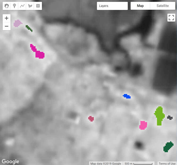
The result is a copy of the input image without the band used to define objects, where pixel values represent the result of the reduction per object, per band (Figure 5).

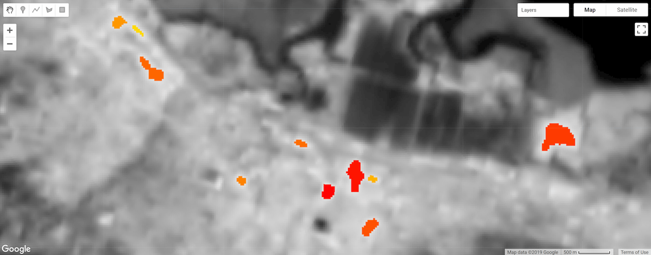
Figure 5. Thermal hotspot object pixels summarized and styled by mean temperature.

Display Earth Engine data layers

Map.addLayerControl()
Map