Book a Demo!
CoCalc Logo Icon
StoreFeaturesDocsShareSupportNewsAboutPoliciesSign UpSign In
polakowo
GitHub Repository: polakowo/vectorbt
Path: blob/master/README.md
1147 views

[!TIP] New in 0.28:

  • Plotly 6 support

  • ticker_kwargs in YFData

  • Fixed Pandas TA dependency (→ pandas-ta-classic).

  • Updated apps and Docker images

đŸ“Ļ Installation

pip install -U vectorbt

To install optional dependencies as well:

pip install -U "vectorbt[full]"

✨ Usage

VectorBT lets you backtest strategies in just a few lines of Python.

  • Profit from investing $100 in Bitcoin since 2014:

import vectorbt as vbt data = vbt.YFData.download("BTC-USD") price = data.get("Close") pf = vbt.Portfolio.from_holding(price, init_cash=100) print(pf.total_profit())
19501.10906763755
  • Buy when the 10-day SMA crosses above the 50-day SMA, and sell on the opposite crossover:

fast_ma = vbt.MA.run(price, 10) slow_ma = vbt.MA.run(price, 50) entries = fast_ma.ma_crossed_above(slow_ma) exits = fast_ma.ma_crossed_below(slow_ma) pf = vbt.Portfolio.from_signals(price, entries, exits, init_cash=100) print(pf.total_profit())
34417.80960086067
  • Generate 1,000 strategies with random signals and test them on BTC and ETH:

import numpy as np symbols = ["BTC-USD", "ETH-USD"] data = vbt.YFData.download(symbols, missing_index="drop") price = data.get("Close") n = np.random.randint(10, 101, size=1000).tolist() pf = vbt.Portfolio.from_random_signals(price, n=n, init_cash=100, seed=42) mean_expectancy = pf.trades.expectancy().groupby(["randnx_n", "symbol"]).mean() fig = mean_expectancy.unstack().vbt.scatterplot(xaxis_title="randnx_n", yaxis_title="mean_expectancy") fig.show()

  • For hyperparameter optimization fans: test 10,000 window combinations of a dual-SMA crossover strategy on BTC, ETH, and XRP:

symbols = ["BTC-USD", "ETH-USD", "XRP-USD"] data = vbt.YFData.download(symbols, missing_index="drop") price = data.get("Close") windows = np.arange(2, 101) fast_ma, slow_ma = vbt.MA.run_combs(price, window=windows, r=2, short_names=["fast", "slow"]) entries = fast_ma.ma_crossed_above(slow_ma) exits = fast_ma.ma_crossed_below(slow_ma) pf = vbt.Portfolio.from_signals(price, entries, exits, size=np.inf, fees=0.001, freq="1D") fig = pf.total_return().vbt.heatmap( x_level="fast_window", y_level="slow_window", slider_level="symbol", symmetric=True, trace_kwargs=dict(colorbar=dict(title="Total return", tickformat="%"))) fig.show()

Inspect any strategy configuration by indexing with pandas:

print(pf[(10, 20, "ETH-USD")].stats())
Start 2017-11-09 00:00:00+00:00 End 2026-01-03 00:00:00+00:00 Period 2978 days 00:00:00 Start Value 100.0 End Value 1604.093789 Total Return [%] 1504.093789 Benchmark Return [%] 866.094127 Max Gross Exposure [%] 100.0 Total Fees Paid 204.226289 Max Drawdown [%] 70.734951 Max Drawdown Duration 1095 days 00:00:00 Total Trades 81 Total Closed Trades 80 Total Open Trades 1 Open Trade PnL -14.232533 Win Rate [%] 41.25 Best Trade [%] 120.511071 Worst Trade [%] -27.772271 Avg Winning Trade [%] 27.265519 Avg Losing Trade [%] -9.022864 Avg Winning Trade Duration 32 days 20:21:49.090909091 Avg Losing Trade Duration 8 days 16:51:03.829787234 Profit Factor 1.275515 Expectancy 18.979079 Sharpe Ratio 0.861945 Calmar Ratio 0.572758 Omega Ratio 1.20277 Sortino Ratio 1.301377 Name: (10, 20, ETH-USD), dtype: object

Same goes for plotting:

pf[(10, 20, "ETH-USD")].plot().show()

It's not all about backtesting! VectorBT can also help with financial data analysis and visualization.

  • Create a GIF that animates Bollinger Bands %B and bandwidth across multiple symbols:

symbols = ["BTC-USD", "ETH-USD", "XRP-USD"] data = vbt.YFData.download(symbols, period="6mo", missing_index="drop") price = data.get("Close") bbands = vbt.BBANDS.run(price) def plot(index, bbands): bbands = bbands.loc[index] fig = vbt.make_subplots( rows=2, cols=1, shared_xaxes=True, vertical_spacing=0.15, subplot_titles=("%B", "Bandwidth")) fig.update_layout(showlegend=False, width=750, height=400) bbands.percent_b.vbt.ts_heatmap( trace_kwargs=dict(zmin=0, zmid=0.5, zmax=1, colorscale="Spectral", colorbar=dict( y=(fig.layout.yaxis.domain[0] + fig.layout.yaxis.domain[1]) / 2, len=0.5 )), add_trace_kwargs=dict(row=1, col=1), fig=fig) bbands.bandwidth.vbt.ts_heatmap( trace_kwargs=dict(colorbar=dict( y=(fig.layout.yaxis2.domain[0] + fig.layout.yaxis2.domain[1]) / 2, len=0.5 )), add_trace_kwargs=dict(row=2, col=1), fig=fig) return fig vbt.save_animation("bbands.gif", bbands.wrapper.index, plot, bbands, delta=90, step=3, fps=3)
100%|██████████| 31/31 [00:21<00:00, 1.21it/s]

This is just the tip of the iceberg. Visit the website to learn more.
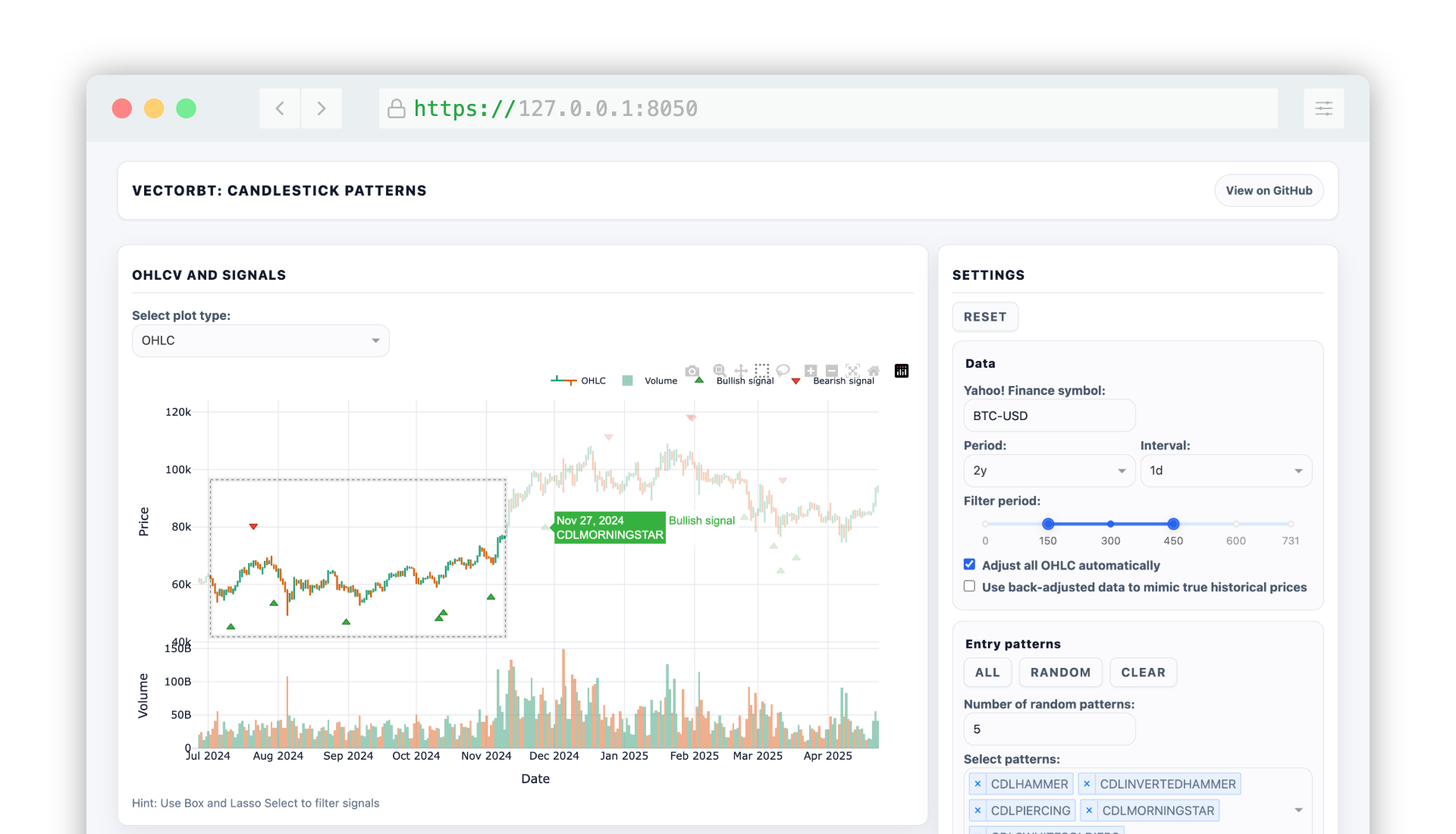
đŸ•šī¸ Apps

Candlestick Patterns (here)

Explore candlestick-pattern signals interactively and backtest them with VectorBT.

teaser.png

âš–ī¸ License

This work is fair-code distributed under the Apache 2.0 with Commons Clause license.

The source code is open, and everyone (individuals and organizations) may use it for free. However, you may not sell products or services that are primarily this software.

If you have questions or want to request a license exception, please contact the author.

Installing optional dependencies may be subject to a more restrictive license.

⭐ Star History

Star History Chart

âš ī¸ Disclaimer

This software is for educational purposes only. Do not risk money you cannot afford to lose.

USE THE SOFTWARE AT YOUR OWN RISK. THE AUTHORS AND ALL AFFILIATES ASSUME NO RESPONSIBILITY FOR YOUR TRADING RESULTS.