sngp_jax.ipynb

Kernel: Python 3.7.11 ('probml')

Uncertainty-aware Deep Learning with SNGP

Author: Nimish Sanghi https://github.com/nsanghi

In this notebook we will use JAX, Flax, Optax and Edward2

JAX - JAX is Autograd and XLA, brought together for high-performance numerical computing and machine learning research. It provides composable transformations of Python+NumPy programs: differentiate, vectorize, parallelize, Just-In-Time compile to GPU/TPU, and more.

Flax - Flax is a neural network library and ecosystem for JAX that is designed for flexibility. Flax is in use by a growing community of researchers and engineers at Google who happily use Flax for their daily research.

Optax - Optax is a gradient processing and optimization library for JAX. It is designed to facilitate research by providing building blocks that can be recombined in custom ways in order to optimise parametric models such as, but not limited to, deep neural networks.

Edward2 - Edward2 is a simple probabilistic programming language. It provides core utilities in deep learning ecosystems so that one can write models as probabilistic programs and manipulate a model's computation for flexible training and inference.

This notebook is based on: https://github.com/tensorflow/docs/blob/master/site/en/tutorials/understanding/sngp.ipynb

In AI applications that are safety-critical, such as medical decision making and autonomous driving, or where the data is inherently noisy (for example, natural language understanding), it is important for a deep classifier to reliably quantify its uncertainty. The deep classifier should be able to be aware of its own limitations and when it should hand control over to the human experts. This tutorial shows how to improve a deep classifier's ability in quantifying uncertainty using a technique called Spectral-normalized Neural Gaussian Process SNGP.

The core idea of SNGP is to improve a deep classifier's distance awareness by applying simple modifications to the network. A model's distance awareness is a measure of how its predictive probability reflects the distance between the test example and the training data. This is a desirable property that is common for gold-standard probabilistic models (for example, the Gaussian process with RBF kernels) but is lacking in models with deep neural networks. SNGP provides a simple way to inject this Gaussian-process behavior into a deep classifier while maintaining its predictive accuracy.

This tutorial implements a deep residual network (ResNet)-based SNGP model on scikit-learn’s two moons dataset.

This tutorial illustrates the SNGP model on a toy 2D dataset.

About SNGP

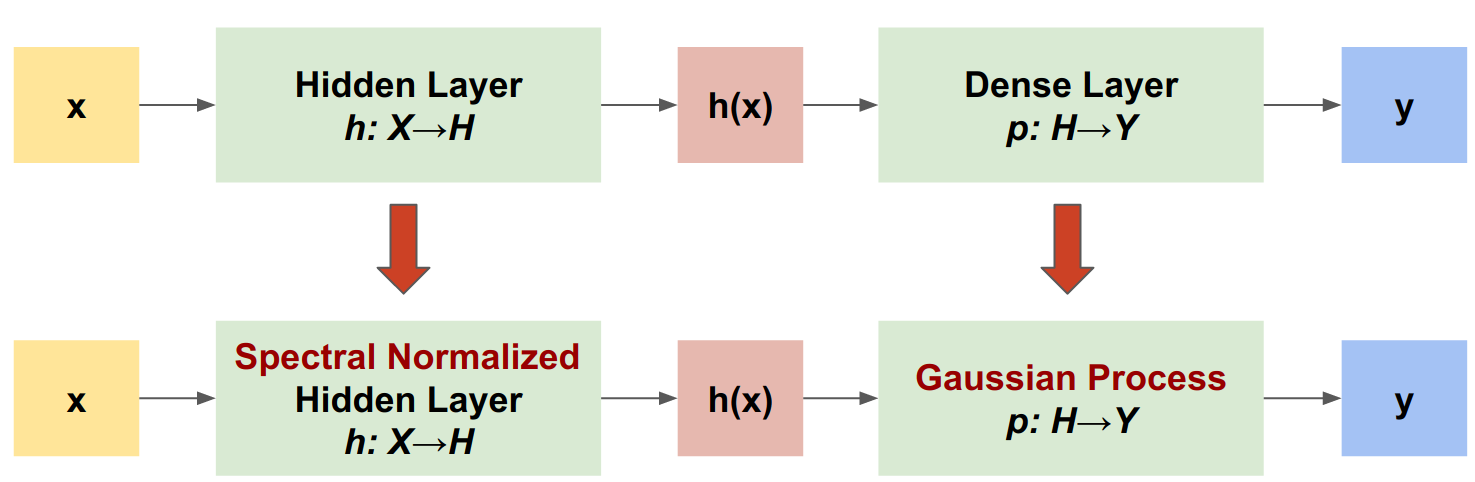
SNGP is a simple approach to improve a deep classifier's uncertainty quality while maintaining a similar level of accuracy and latency. Given a deep residual network, SNGP makes two simple changes to the model:

• It applies spectral normalization to the hidden residual layers.

• It replaces the Dense output layer with a Gaussian process layer.

Compared to other uncertainty approaches (such as Monte Carlo dropout or Deep ensemble), SNGP has several advantages:

• It works for a wide range of state-of-the-art residual-based architectures (for example, (Wide) ResNet, DenseNet, or BERT).

• It is a single-model method—it does not rely on ensemble averaging). Therefore, SNGP has a similar level of latency as a single deterministic network, and can be scaled easily to large datasets like ImageNet and Jigsaw Toxic Comments classification

• It has strong out-of-domain detection performance due to the distance-awareness property.

The downsides of this method are:

• The predictive uncertainty of SNGP is computed using the Laplace approximation. Therefore, theoretically, the posterior uncertainty of SNGP is different from that of an exact Gaussian process.

• SNGP training needs a covariance reset step at the beginning of a new epoch. This can add a tiny amount of extra complexity to a training pipeline. This tutorial shows a simple way to implement this using direct update of state of the model.

# Imports
%matplotlib inline
import matplotlib.pyplot as plt
import matplotlib.colors as colors
import jax
import jax.numpy as jnp
import numpy as np
import functools
from typing import Any, Callable, Iterable, Mapping, Optional, Tuple, Union
from jax import random

linalg = jax.lax.linalg

# Jax-related data types.
Axes = Union[int, Iterable[int]]
PRNGKey = Any
Shape = Iterable[int]
Dtype = type(jnp.float32)
Array = jnp.ndarray
Initializer = Callable[[PRNGKey, Shape, Dtype], Array]

try:
    import sklearn.datasets
except ModuleNotFoundError:
    %pip install -qq -U scikit-learn
    import sklearn.datasets

try:
    import flax
    import flax.linen as nn
    from flax.training import train_state
except ModuleNotFoundError:
    %pip install -qq -U flax
    import flax
    import flax.linen as nn
    from flax.training import train_state

try:
    import optax
except ModuleNotFoundError:
    %pip install -qq -U optax
    import optax

try:
    import edward2.jax as ed
except ModuleNotFoundError:
    %pip install -qq -U "git+https://github.com/google/edward2.git#egg=edward2"
    import edward2.jax as ed

     |████████████████████████████████| 180 kB 28.9 MB/s 
     |████████████████████████████████| 1.0 MB 60.3 MB/s 
     |████████████████████████████████| 217 kB 69.9 MB/s 
     |████████████████████████████████| 145 kB 76.2 MB/s 
     |████████████████████████████████| 51 kB 9.7 MB/s 
     |████████████████████████████████| 76 kB 7.1 MB/s 
  Building wheel for jax (setup.py) ... done
  Building wheel for edward2 (setup.py) ... done

Define visualization macros

plt.rcParams["figure.dpi"] = 140

DEFAULT_X_RANGE = (-3.5, 3.5)
DEFAULT_Y_RANGE = (-2.5, 2.5)
DEFAULT_CMAP = colors.ListedColormap(["#377eb8", "#ff7f00"])
DEFAULT_NORM = colors.Normalize(
    vmin=0,
    vmax=1,
)
DEFAULT_N_GRID = 100

The two moon dataset

Create the training and evaluation datasets from the scikit-learn two moon dataset.

def make_training_data(sample_size=500):
    """Create two moon training dataset."""
    train_examples, train_labels = sklearn.datasets.make_moons(n_samples=2 * sample_size, noise=0.1)

    # Adjust data position slightly.
    train_examples[train_labels == 0] += [-0.1, 0.2]
    train_examples[train_labels == 1] += [0.1, -0.2]

    return train_examples, train_labels

Evaluate the model's predictive behavior over the entire 2D input space.

def make_testing_data(x_range=DEFAULT_X_RANGE, y_range=DEFAULT_Y_RANGE, n_grid=DEFAULT_N_GRID):
    """Create a mesh grid in 2D space."""
    # testing data (mesh grid over data space)
    x = np.linspace(x_range[0], x_range[1], n_grid)
    y = np.linspace(y_range[0], y_range[1], n_grid)
    xv, yv = np.meshgrid(x, y)
    return np.stack([xv.flatten(), yv.flatten()], axis=-1)

To evaluate model uncertainty, add an out-of-domain (OOD) dataset that belongs to a third class. The model never observes these OOD examples during training.

def make_ood_data(sample_size=500, means=(2.5, -1.75), vars=(0.01, 0.01)):
    return np.random.multivariate_normal(means, cov=np.diag(vars), size=sample_size)

# Load the train, test and OOD datasets.
train_examples, train_labels = make_training_data(sample_size=500)
test_examples = make_testing_data()
ood_examples = make_ood_data(sample_size=500)

# Visualize
pos_examples = train_examples[train_labels == 0]
neg_examples = train_examples[train_labels == 1]

plt.figure(figsize=(7, 5.5))

plt.scatter(pos_examples[:, 0], pos_examples[:, 1], c="#377eb8", alpha=0.5)
plt.scatter(neg_examples[:, 0], neg_examples[:, 1], c="#ff7f00", alpha=0.5)
plt.scatter(ood_examples[:, 0], ood_examples[:, 1], c="red", alpha=0.1)

plt.legend(["Positive", "Negative", "Out-of-Domain"])

plt.ylim(DEFAULT_Y_RANGE)
plt.xlim(DEFAULT_X_RANGE)

plt.show()

Here, the blue and orange represent the positive and negative classes, and the red represents the OOD data. A model that quantifies the uncertainty well is expected to be confident when close to training data (i.e., $p(x_{test})$ close to 0 or 1), and be uncertain when far away from the training data regions (i.e., $p(x_{test})$ close to 0.5).

The deterministic model

Define model

Start from the (baseline) deterministic model: a multi-layer residual network (ResNet) with dropout regularization.

class DeepResNet(nn.Module):
    num_classes: int
    num_layers: int = 3
    num_hidden: int = 128
    dropout_rate: float = 0.1

    @nn.compact
    def __call__(self, inputs, train):
        # ResNet
        x = inputs
        hidden = nn.Dense(self.num_hidden, name="input_layer")(x)
        hidden = jax.lax.stop_gradient(hidden)
        for i in range(self.num_layers):
            resid = nn.Dense(self.num_hidden, name=f"dense_layers_{i}")(hidden)
            resid = nn.relu(resid)
            resid = nn.Dropout(self.dropout_rate)(resid, deterministic=not train)
            hidden += resid
        out = nn.Dense(self.num_classes, name="classifier")(hidden)
        return out

This tutorial uses a six-layer ResNet with 128 hidden units.

resnet_config = dict(num_classes=2, num_layers=6, num_hidden=128)

Define Loss and metrics

def cross_entropy_loss(*, logits, labels):
    labels_onehot = jax.nn.one_hot(labels, num_classes=2)
    return optax.softmax_cross_entropy(logits=logits, labels=labels_onehot).mean()


def compute_metrics(*, logits, labels):
    loss = cross_entropy_loss(logits=logits, labels=labels)
    accuracy = jnp.mean(jnp.argmax(logits, -1) == labels)
    metrics = {
        "loss": loss,
        "accuracy": accuracy,
    }
    return metrics

Create train state

A common pattern in Flax is to create a single dataclass that represents the entire training state, including step number, parameters, and optimizer state.

def create_train_state(rng, learning_rate, model):
    """Creates initial `TrainState`."""
    # resnet_model = DeepResNet(**resnet_config)
    params = model.init(rng, jnp.ones([1, 2]), train=True)["params"]
    tx = optax.adam(learning_rate)
    return train_state.TrainState.create(apply_fn=model.apply, params=params, tx=tx)

Train Step

A function that:

• Evaluates the neural network given the parameters and a batch of input images with the Module.apply method.

• Computes the cross_entropy_loss loss function.

• Evaluates the loss function and its gradient using jax.value_and_grad.

• Applies a pytree of gradients to the optimizer to update the model’s parameters.

• Computes the metrics using compute_metrics (defined earlier).

Use JAX’s @jit decorator to trace the entire train_step function and just-in-time compile it with XLA into fused device operations that run faster and more efficiently on hardware accelerators.

@jax.jit
def train_step(state, batch, rng):
    """Train for a single step."""

    def loss_fn(params):
        logits = state.apply_fn({"params": params}, batch["input"], train=True, rngs={"dropout": rng})
        loss = cross_entropy_loss(logits=logits, labels=batch["label"])
        return loss, logits

    grad_fn = jax.value_and_grad(loss_fn, has_aux=True)
    (_, logits), grads = grad_fn(state.params)
    state = state.apply_gradients(grads=grads)
    metrics = compute_metrics(logits=logits, labels=batch["label"])
    return state, metrics


@jax.jit
def get_prob(state, batch):
    logits = state.apply_fn({"params": state.params}, batch, train=False)
    probs = nn.softmax(logits)
    return probs

Train Function

def train_epoch(state, train_ds, batch_size, epoch, rng):
    """Train for a single epoch."""
    train_ds_size = len(train_ds["input"])
    steps_per_epoch = train_ds_size // batch_size

    rng, dropout_rng = jax.random.split(rng)
    perms = jax.random.permutation(rng, train_ds_size)
    perms = perms[: steps_per_epoch * batch_size]  # skip incomplete batch
    perms = perms.reshape((steps_per_epoch, batch_size))
    batch_metrics = []
    for perm in perms:
        dropout_rng, sub_rng = jax.random.split(dropout_rng)
        batch = {"input": train_ds["input"][perm, ...], "label": train_ds["label"][perm]}
        state, metrics = train_step(state, batch, sub_rng)
        batch_metrics.append(metrics)

    # compute mean of metrics across each batch in epoch.
    batch_metrics_np = jax.device_get(batch_metrics)
    epoch_metrics_np = {k: np.mean([metrics[k] for metrics in batch_metrics_np]) for k in batch_metrics_np[0]}

    if epoch % 10 == 0:
        print(
            "train epoch: %d, loss: %.4f, accuracy: %.2f"
            % (epoch, epoch_metrics_np["loss"], epoch_metrics_np["accuracy"] * 100)
        )

    return state

Initialize the state

rng = jax.random.PRNGKey(0)
rng, params_rng, dropout_rng = jax.random.split(rng, num=3)
resnet_model = DeepResNet(**resnet_config)
init_rngs = {"params": params_rng, "dropout": dropout_rng}

learning_rate = 1e-4
state = create_train_state(init_rngs, learning_rate, resnet_model)
del params_rng, dropout_rng, init_rngs

Train the model

num_epochs = 100
batch_size = 128

train_ds = {"input": train_examples, "label": train_labels}

for epoch in range(1, num_epochs + 1):
    # Use a separate PRNG key to permute data during shuffling
    rng, input_rng = jax.random.split(rng)
    # Run an optimization step over a training batch
    state = train_epoch(state, train_ds, batch_size, epoch, input_rng)

train epoch: 10, loss: 0.1069, accuracy: 94.53
train epoch: 20, loss: 0.0967, accuracy: 94.75
train epoch: 30, loss: 0.0893, accuracy: 94.75
train epoch: 40, loss: 0.0849, accuracy: 95.09
train epoch: 50, loss: 0.0811, accuracy: 94.98
train epoch: 60, loss: 0.0661, accuracy: 96.09
train epoch: 70, loss: 0.0672, accuracy: 95.87
train epoch: 80, loss: 0.0573, accuracy: 96.54
train epoch: 90, loss: 0.0540, accuracy: 97.32
train epoch: 100, loss: 0.0490, accuracy: 97.88

Visualize uncertainty

def plot_uncertainty_surface(test_uncertainty, ax, cmap=None):
    """Visualizes the 2D uncertainty surface.

    For simplicity, assume these objects already exist in the memory:

        test_examples: Array of test examples, shape (num_test, 2).
        train_labels: Array of train labels, shape (num_train, ).
        train_examples: Array of train examples, shape (num_train, 2).

    Arguments:
        test_uncertainty: Array of uncertainty scores, shape (num_test,).
        ax: A matplotlib Axes object that specifies a matplotlib figure.
        cmap: A matplotlib colormap object specifying the palette of the
          predictive surface.

    Returns:
        pcm: A matplotlib PathCollection object that contains the palette
          information of the uncertainty plot.
    """
    # Normalize uncertainty for better visualization.
    test_uncertainty = test_uncertainty / np.max(test_uncertainty)

    # Set view limits.
    ax.set_ylim(DEFAULT_Y_RANGE)
    ax.set_xlim(DEFAULT_X_RANGE)

    # Plot normalized uncertainty surface.
    pcm = ax.imshow(
        np.reshape(test_uncertainty, [DEFAULT_N_GRID, DEFAULT_N_GRID]),
        cmap=cmap,
        origin="lower",
        extent=DEFAULT_X_RANGE + DEFAULT_Y_RANGE,
        vmin=DEFAULT_NORM.vmin,
        vmax=DEFAULT_NORM.vmax,
        interpolation="bicubic",
        aspect="auto",
    )

    # Plot training data.
    ax.scatter(train_examples[:, 0], train_examples[:, 1], c=train_labels, cmap=DEFAULT_CMAP, alpha=0.5)
    ax.scatter(ood_examples[:, 0], ood_examples[:, 1], c="red", alpha=0.1)

    return pcm

Now visualize the predictions of the deterministic model. First plot the class probability: $$p(x) = softmax(logit(x))$$

resnet_probs = get_prob(state, test_examples)
resnet_probs_0 = resnet_probs[:, 0]  # Take the probability for class 0.

_, ax = plt.subplots(figsize=(7, 5.5))

pcm = plot_uncertainty_surface(resnet_probs_0, ax=ax)

plt.colorbar(pcm, ax=ax)
plt.title("Class Probability, Deterministic Model")

plt.show()

In this plot, the yellow and purple are the predictive probabilities for the two classes. The deterministic model did a good job in classifying the two known classes—blue and orange—with a nonlinear decision boundary. However, it is not distance-aware, and classified the never-observed red out-of-domain (OOD) examples confidently as the orange class.

Visualize the model uncertainty by computing the predictive variance: $$var(x) = p(x) * (1 - p(x))$$

resnet_uncertainty = resnet_probs_0 * (1 - resnet_probs_0)

_, ax = plt.subplots(figsize=(7, 5.5))

pcm = plot_uncertainty_surface(resnet_uncertainty, ax=ax)

plt.colorbar(pcm, ax=ax)
plt.title("Predictive Uncertainty, Deterministic Model")

plt.show()

In this plot, the yellow indicates high uncertainty, and the purple indicates low uncertainty. A deterministic ResNet's uncertainty depends only on the test examples' distance from the decision boundary. This leads the model to be over-confident when out of the training domain. The next section shows how SNGP behaves differently on this dataset.

The SNGP model

Define SNGP model

Let's now implement the SNGP model. Both the SNGP components, SpectralNormalization and RandomFeatureGaussianProcess, are available in Edward2.

Let's inspect these two components in more detail.

SpectralNormalization wrapper

SpectralNormalization is a Jax layer wrapper in Edward2 library. It can be applied to an existing Dense layer like this:

dense = nn.Dense(features=10)
dense = ed.nn.SpectralNormalization(dense, norm_multiplier=0.9)

Spectral normalization regularizes the hidden weight $W$ by gradually guiding its spectral norm (that is, the largest eigenvalue of $W$) toward the target value norm_multiplier).

Note: Usually it is preferable to set norm_multiplier to a value smaller than 1. However in practice, it can be also relaxed to a larger value to ensure the deep network has enough expressive power.

Next code cell has a simplied implementation of the Spectral Normalization code from Edwards2 library referenced above.

# implementation based on the code contianed in edwards library
# https://github.com/google/edward2/blob/main/edward2/jax/nn/normalization.py
# Below implementaiton is a simplification of the above code


def _l2_normalize(x, eps=1e-12):
    """Normalizes a vector"""
    return x * jax.lax.rsqrt(jnp.maximum(jnp.square(x).sum(), eps))


class SpectralNormalization(nn.Module):
    """Implements spectral normalization for linear layers.
    In Flax, parameters are immutable so we cannot modify the parameters of
    the input layer during the transformation. As a resolution, we will move
    all parameters of the input layer to this spectral normalization layer.
    During the transformation, we will modify the weight and call the input
    layer with the updated weight.
    For example, the pattern for parameters with a Dense input layer will be
      {"Dense": {"weight": ..., "bias": ...}}
    which matches the pattern in Flax as if "Dense" is a submodule of this
    spectral normalization layer.
    Attributes:
        layer: a Flax layer to apply normalization to.
        iteration: the number of power iterations to estimate weight matrix's
          singular value.
        norm_multiplier: multiplicative constant to threshold the normalization.
          Usually under normalization, the singular value will converge to this
          value.
    """

    layer: nn.Module
    iteration: int = 1
    norm_multiplier: float = 0.95
    u_init: Callable[[PRNGKey, Shape, Dtype], Array] = nn.initializers.normal(stddev=0.05)
    v_init: Callable[[PRNGKey, Shape, Dtype], Array] = nn.initializers.normal(stddev=0.05)
    kernel_apply_kwargs: Optional[Mapping[str, Any]] = None

    # weight vector `w` is named as `kernel` in the Flax implementation
    # of the `Dense` layer
    kernel_name: str = "kernel"

    # to initialize the spectral variables u and v first time
    # and return the same subsequently
    def _get_singular_vectors(self, initializing, kernel_apply, in_shape, dtype):
        if initializing:
            rng_u = self.make_rng("params")
            rng_v = self.make_rng("params")
            # Interpret output shape (not that this does not cost any FLOPs).
            out_shape = jax.eval_shape(kernel_apply, jax.ShapeDtypeStruct(in_shape, dtype)).shape
        else:
            rng_u = rng_v = out_shape = None
        u = self.variable("spectral_stats", "u", self.u_init, rng_u, out_shape, dtype)
        v = self.variable("spectral_stats", "v", self.v_init, rng_v, in_shape, dtype)
        return u, v

    @nn.compact
    def __call__(self, inputs: Array, training: bool = True) -> Array:
        """Applies a linear transformation with spectral normalization to the inputs.
        Args:
            inputs: The nd-array to be transformed.
            training: Whether to perform power interations to update the singular
              value estimate.
        Returns:
            The transformed input.
        """
        layer_name = type(self.layer).__name__
        params = self.param(layer_name, lambda *args: self.layer.init(*args)["params"], inputs)
        w = params[self.kernel_name]

        kernel_apply = lambda x: x @ w.reshape(-1, w.shape[-1])
        in_shape = (np.prod(w.shape[:-1]),)

        initializing = self.is_mutable_collection("params")
        u, v = self._get_singular_vectors(initializing, kernel_apply, in_shape, w.dtype)
        u_hat, v_hat = u.value, v.value
        u_, kernel_transpose = jax.vjp(kernel_apply, v_hat)
        if training and not initializing:
            # Run power iterations using autodiff approach.
            # https://arxiv.org/pdf/1802.05957v1.pdf - Appendix A Page 15
            # https://nbviewer.org/gist/shoyer/fa9a29fd0880e2e033d7696585978bfc
            def scan_body(carry, _):
                u_hat, v_hat, u_ = carry
                (v_,) = kernel_transpose(u_hat)
                v_hat = _l2_normalize(v_)
                u_ = kernel_apply(v_hat)
                u_hat = _l2_normalize(u_)
                return (u_hat, v_hat, u_), None

            (u_hat, v_hat, u_), _ = jax.lax.scan(scan_body, (u_hat, v_hat, u_), None, length=self.iteration)
            u.value, v.value = u_hat, v_hat

        sigma = jnp.vdot(u_hat, u_)
        # Bound spectral norm by the `norm_multiplier`.
        sigma = jnp.maximum(sigma / self.norm_multiplier, 1.0)
        w_hat = w / jax.lax.stop_gradient(sigma)
        self.sow("intermediates", "w", w_hat)

        # Update params.
        params = flax.core.unfreeze(params)
        params[self.kernel_name] = w_hat
        layer_params = flax.core.freeze({"params": params})
        return self.layer.apply(layer_params, inputs)

The Gaussian Process (GP) layer

SNGP replaces the typical dense output layer with a Gaussian process (GP) with an RBF kernel, whose posterior variance at $x^∗$ is characterized by its $L_2$ distance from the training data in the hidden space.

RandomFeatureGaussianProcess implements a random-feature based approximation to a Gaussian process model that is end-to-end trainable with a deep neural network. Under the hood, the Gaussian process layer implements a two-layer network:

$$logits(x) = \Phi(x) \beta, \quad \Phi(x)=\sqrt{\frac{2}{M}} * cos(Wx + b)$$

Here, $x$ is the input, and $W$ and $b$ are frozen weights initialized randomly from Gaussian and Uniform distributions, respectively. (Therefore, $\Phi(x)$ are called "random features".) $\beta$ is the learnable kernel weight similar to that of a Dense layer.

batch_size = 32
hidden_features = 1024
num_classes = 10

hidden_kwargs = {"feature_scale": None}
covmat_kwargs = {"momentum": None}

gp_layer = ed.nn.RandomFeatureGaussianProcess(
    features=num_classes,
    hidden_features=hidden_features,
    normalize_input=False,
    hidden_kwargs=hidden_features,
    covmat_kwargs=covmat_kwargs,
)

The main parameters of the GP layers are:

• features: The dimension of the output logits.

• num_inducing: The dimension $M$ of the hidden weight $W$. Default to 1024.

• normalize_input: Whether to apply layer normalization to the input $x$.

• feature_scale: Defined in hidden_kwargs. Use None to apply the scale $\sqrt{2/M}$ to the hidden output.

• momentum: Defined in covmat_kwargs. The momentum of the kernel weight update. Default to None.

Note: For a deep neural network that is sensitive to the learning rate (for example, ResNet-50 and ResNet-110), it is generally recommended to set normalize_input=True to stabilize training, and set feature_scale=1. to avoid the learning rate from being modified in unexpected ways when passing through the GP layer.

• momentum controls how the model covariance is computed. If set to a positive value (for example, 0.999), the covariance matrix is computed using the momentum-based moving average update (similar to batch normalization). If set to None, the covariance matrix is updated without momentum.

Note: The momentum-based update method can be sensitive to batch size. Therefore it is generally recommended to set momentum=None to compute the covariance exactly. For this to work properly, the covariance matrix estimator needs to be reset at the beginning of a new epoch in order to avoid counting the same data twice. precision_matrix is the state of the RandomFeatureGaussianProcess layer which we need to access and reset at the begining of each epoch. Function defined below reset_precision_matrix(state) resets the covariance matrix estimator to an Identity matrix.

Given a batch input with shape (batch_size, input_dim), the GP layer returns a logits tensor (shape (batch_size, num_classes)) for prediction, and also covmat tensor (shape (batch_size,) or (batch_size, batch_size)) which is the posterior covariance matrix of the batch logits.

In the code cells below, we implement a simplified version of RandomFeatureGaussianProcess by borrowing the original code from Edwards2 library and removing various configurtaiton settings not relevant to this demonstration as well as hard-coding some of the above recommended settings.

Self Contained Implementation of SNGP layers

RandomFourierFeatures

Code cell implements random features as per equation (6) of the SNGP paper.

The only difference is that as recommended, the code uses a feature_scale of 1 instead of $\sqrt{2/M}$

$$\Phi(x)=\sqrt{\frac{2}{M}} * cos(Wx + b)$$

where, entries in matrix $W$ is sampled from $N(0,1)$ and entries in $b$ are sampled from $Uniform(0,2\pi)$. These are sampled in the begining and then fixed. These are not trainable parameters.

# Default config for random features.
default_rbf_activation = jnp.cos
default_rbf_bias_init = nn.initializers.uniform(scale=2.0 * jnp.pi)
# Using "he_normal" style random feature distribution. Effectively, this is
# equivalent to approximating a RBF kernel but with the input standardized by
# its dimensionality (i.e., input_scaled = input * sqrt(2. / dim_input)) and
# empirically leads to better performance for neural network inputs.
default_rbf_kernel_init = nn.initializers.variance_scaling(scale=2.0, mode="fan_in", distribution="normal")


class RandomFourierFeatures(nn.Module):
    """A random fourier feature (RFF) layer that approximates a kernel model.
    The random feature transformation is a one-hidden-layer network with
    non-trainable weights. Specifically:
    f(x) = activation(x @ kernel + bias) * output_scale (output_scale = 1 in this demo).
    The forward pass logic closely follows that of the nn.Dense.
    Attributes:
      features: the number of output units.
      seed: random seed for generating random features (default: 0). This will
        override the external RNGs.
      dtype: the dtype of the computation (default: float32).
    """

    features: int
    seed: int = 0
    dtype: Dtype = jnp.float32
    collection_name: str = "random_features"

    def setup(self):
        # Defines the random number generator.
        self.rng = random.PRNGKey(self.seed)

        # Processes random feature scale.
        self._feature_scale = 1.0
        self._feature_scale = jnp.asarray(self._feature_scale, dtype=self.dtype)

    @nn.compact
    def __call__(self, inputs: Array) -> Array:
        input_dim = inputs.shape[-1]

        kernel_rng, bias_rng = random.split(self.rng, num=2)
        kernel_shape = (input_dim, self.features)

        kernel = self.variable(
            self.collection_name, "kernel", default_rbf_kernel_init, kernel_rng, kernel_shape, self.dtype
        )
        bias = self.variable(
            self.collection_name, "bias", default_rbf_bias_init, bias_rng, (self.features,), self.dtype
        )

        # Specifies multiplication dimension.
        contracting_dims = ((inputs.ndim - 1,), (0,))
        batch_dims = ((), ())

        # Performs forward pass.
        inputs = jnp.asarray(inputs, self.dtype)
        outputs = jax.lax.dot_general(inputs, kernel.value, (contracting_dims, batch_dims))
        outputs = outputs + jnp.broadcast_to(bias.value, outputs.shape)

        return self._feature_scale * default_rbf_activation(outputs)

LaplaceRandomFeatureCovariance

Notice that under this implementation of the SNGP model as well as in Edwards2 library , the predictive logits for all classes share the same covariance matrix , which describes the distance between from the training data.

Theoretically, it is possible to extend the algorithm to compute different variance values for different classes (as introduced in the original SNGP paper. However, this is difficult to scale to problems with large output spaces (such as classification with ImageNet or language modeling).

class LaplaceRandomFeatureCovariance(nn.Module):
    """Computes the Gaussian Process covariance using Laplace method.

    Attributes:
      hidden_features: the number of random fourier features.
    """

    hidden_features: int
    collection_name: str = "laplace_covariance"
    dtype: Dtype = jnp.float32

    def compute_predictive_covariance(
        self, gp_features: Array, precision_matrix: nn.Variable, diagonal_only: bool
    ) -> Array:
        """Computes the predictive covariance.

        Approximates the Gaussian process posterior using random features.
        Given training random feature `Phi_tr (num_train, num_hidden)` and `testing
        random feature Phi_ts (batch_size, num_hidden)`. The predictive `covariance`
        matrix is computed as:

        s * Phi_ts @ inv(t(Phi_tr) * Phi_tr + s * I) @ t(Phi_ts),

        where s is the ridge factor to be used for stablizing the inverse, and I is
        the identity matrix with shape (num_hidden, num_hidden). The above
        description is formal only: the actual implementation uses a Cholesky
        factorization of the covariance matrix t(Phi_tr) * Phi_tr + s * I.

        Args:
          gp_features: the random feature of testing data to be used for computing
            the covariance matrix. Shape (batch_size, gp_hidden_size).
          precision_matrix: the model'`s precision matrix.
          diagonal_only: whether to return only the diagonal elements of the
            predictive covariance matrix (i.e., the predictive variances).

        Returns:
          The predictive variances of shape (batch_size, ) if diagonal_only=True,
          otherwise the predictive covariance matrix of shape
          (batch_size, batch_size)

        """

        chol = linalg.cholesky(precision_matrix.value)
        chol_t_cov_feature_product = linalg.triangular_solve(chol, gp_features.T, left_side=True, lower=True)

        if diagonal_only:
            # Compute diagonal element only, shape (batch_size, ).
            gp_covar = jnp.square(chol_t_cov_feature_product).sum(0)
        else:
            # Compute full covariance matrix, shape (batch_size, batch_size).
            gp_covar = chol_t_cov_feature_product.T @ chol_t_cov_feature_product

        return gp_covar

    @nn.compact
    def __call__(self, gp_features: Array, diagonal_only: bool = True) -> Optional[Array]:

        """Updates the precision matrix and computes the predictive covariance.

        NOTE:
        The precision matrix will be updated only during training (i.e., when
        `self.collection_name` are in the list of mutable variables). The covariance
        matrix will be computed only during inference to avoid repeated calls to the
        (expensive) `linalg.inv` op.

        Args:
          gp_features: The nd-array of random fourier features, shape (batch_size,
            ..., hidden_features).
          diagonal_only: Whether to return only the diagonal elements of the
            predictive covariance matrix (i.e., the predictive variance).

        Returns:
          The predictive variances of shape (batch_size, ) if diagonal_only=True,
          otherwise the predictive covariance matrix of shape
          (batch_size, batch_size).
        """
        gp_features = jnp.asarray(gp_features, self.dtype)

        # Flatten GP features and logits to 2-d, by doing so we treat all the
        # non-final dimensions as the batch dimensions.
        gp_features = jnp.reshape(gp_features, [-1, self.hidden_features])

        precision_matrix = self.variable(
            self.collection_name, "precision_matrix", lambda: self.initial_precision_matrix()
        )  # pylint: disable=unnecessary-lambda

        # Updates the precision matrix during training.
        initializing = self.is_mutable_collection("params")
        training = self.is_mutable_collection(self.collection_name)

        if training and not initializing:
            precision_matrix.value = self.update_precision_matrix(gp_features, precision_matrix.value)

        # Computes covariance matrix during inference.
        if not training:
            return self.compute_predictive_covariance(gp_features, precision_matrix, diagonal_only)

    def initial_precision_matrix(self):
        """Returns the initial diagonal precision matrix."""
        return jnp.eye(self.hidden_features, dtype=self.dtype)

    def update_precision_matrix(self, gp_features: Array, precision_matrix: Array) -> Array:
        """Updates precision matrix given a new batch.

        Args:
          gp_features: random features from the new batch, shape (batch_size,
            hidden_features)
          precision_matrix: the current precision matrix, shape (hidden_features,
            hidden_features).

        Returns:
          Updated precision matrix, shape (hidden_features, hidden_features).
        """

        batch_prec_mat = jnp.matmul(jnp.transpose(gp_features), gp_features)

        # Updates precision matrix.
        # Performs exact update without momentum.
        precision_matrix_updated = precision_matrix + batch_prec_mat

        return precision_matrix_updated

RandomFeatureGaussianProcess

Implementation below finally uses the above two functions RandomFourierFeatures and LaplaceRandomFeatureCovariance to implement the distance aware output layer using GP

The hidden features from the last spectral normaized layer in the pipeline are passed through a RandomFoureirFeatures and then a dense layer to get the MAP estimate of logits. These are then passed through LaplaceRandomFeatureCovariance to calculate the posterior covariance of the GP.

class RandomFeatureGaussianProcess(nn.Module):
    """A Gaussian process layer using random Fourier features [1].
    Attributes:
      features: the number of output units.
      hidden_features: the number of hidden random fourier features.
      normalize_input: whether to normalize the input using nn.LayerNorm.
      norm_kwargs: Optional keyword arguments to the input nn.LayerNorm layer.
      hidden_kwargs: Optional keyword arguments to the random feature layer.
      output_kwargs: Optional keyword arguments to the predictive logit layer.
      covmat_kwargs: Optional keyword arguments to the predictive covmat layer.
    """

    features: int
    hidden_features: int = 1024
    normalize_input: bool = True

    def setup(self):
        """Defines model layers."""
        # pylint:disable=invalid-name,not-a-mapping
        if self.normalize_input:
            LayerNorm = functools.partial(nn.LayerNorm, use_bias=False, use_scale=False)
            self.norm_layer = LayerNorm(**self.norm_kwargs)

        self.hidden_layer = RandomFourierFeatures(features=self.hidden_features)

        self.output_layer = nn.Dense(features=self.features)
        self.covmat_layer = LaplaceRandomFeatureCovariance(hidden_features=self.hidden_features)
        # pylint:enable=invalid-name,not-a-mapping

    def __call__(self, inputs: Array, return_full_covmat: bool = False, return_random_features: bool = False) -> Array:
        """Computes Gaussian process outputs.
        Args:
          inputs: the nd-array of shape (batch_size, ..., input_dim).
          return_full_covmat: whether to return the full covariance matrix, shape
            (batch_size, batch_size), or only return the predictive variances with
            shape (batch_size, ).
          return_random_features: whether to return the random fourier features for
            the inputs.
        Returns:
          A tuple of predictive logits, predictive covmat and (optionally)
          random Fourier features.
        """
        gp_inputs = self.norm_layer(inputs) if self.normalize_input else inputs
        gp_features = self.hidden_layer(gp_inputs)

        gp_logits = self.output_layer(gp_features)
        gp_covmat = self.covmat_layer(gp_features, diagonal_only=not return_full_covmat)

        # Returns predictive logits, covmat and (optionally) random features.
        if return_random_features:
            return gp_logits, gp_covmat, gp_features
        return gp_logits, gp_covmat

The full SNGP model

Given the base class DeepResNet, the SNGP model can be implemented easily by modifying the residual network's hidden and output layers.

class DeepResNetSNGP(nn.Module):
    num_classes: int
    num_layers: int = 3
    num_hidden: int = 128
    dropout_rate: float = 0.1
    spec_norm_bound: float = 0.9

    @nn.compact
    def __call__(self, inputs, training=False):
        # ResNet
        x = inputs
        hidden = nn.Dense(self.num_hidden, name="input_layer")(x)
        hidden = jax.lax.stop_gradient(hidden)
        for i in range(self.num_layers):
            # in line below use `ed.nn.SpectralNormalization` to
            # use implementation from `edwards2` library
            resid = SpectralNormalization(nn.Dense(self.num_hidden), norm_multiplier=self.spec_norm_bound)(
                hidden, training=training
            )
            resid = nn.relu(resid)
            resid = nn.Dropout(self.dropout_rate)(resid, deterministic=not training)
            hidden += resid
            # in line below use `ed.nn.RandomFeatureGaussianProcess` to
            # use implementation from `edwards2` library
        logits, covmat = RandomFeatureGaussianProcess(features=self.num_classes, normalize_input=False)(hidden)
        if not training:
            return logits, covmat
        return logits

Update Step

Next we define update_step which implements a single step of model update. As we need to split the variables into two categories state, the internal state of the model and params, the model's parameters which are updated by the optimizer. state gets updated internally as part of the training step and are required to be extracted and fed back again at the next iteration. And params are the parameters that are updated by the optimizer.

def update_step(apply_fn, batch, opt_state, params, state, tx, rng):
    def loss_fn(params):
        logits, updated_state = apply_fn(
            {"params": params, **state},
            batch["input"],
            rngs={"dropout": rng},
            training=True,
            mutable=list(state.keys()),
        )
        loss = cross_entropy_loss(logits=logits, labels=batch["label"])
        metrics = compute_metrics(logits=logits, labels=batch["label"])
        return loss, (metrics, updated_state)

    (loss, (metrics, updated_state)), grads = jax.value_and_grad(loss_fn, has_aux=True)(params)
    updates, opt_state = tx.update(grads, opt_state)  # Defined below.
    params = optax.apply_updates(params, updates)
    return metrics, opt_state, params, updated_state

Training over one epoch

THe code below implements a single step through the full training data, shuffling the data at the beginning of each epoch.

def train_epoch_sngp(apply_fn, opt_state, params, state, tx, train_ds, batch_size, epoch, rng):
    """Train for a single epoch."""
    train_ds_size = len(train_ds["input"])
    steps_per_epoch = train_ds_size // batch_size

    rng, dropout_rng = jax.random.split(rng)
    perms = jax.random.permutation(rng, train_ds_size)
    perms = perms[: steps_per_epoch * batch_size]  # skip incomplete batch
    perms = perms.reshape((steps_per_epoch, batch_size))
    batch_metrics = []
    for perm in perms:
        dropout_rng, sub_rng = jax.random.split(dropout_rng)
        batch = {"input": train_ds["input"][perm, ...], "label": train_ds["label"][perm]}
        metrics, opt_state, params, state = update_step(apply_fn, batch, opt_state, params, state, tx, sub_rng)
        batch_metrics.append(metrics)

    # compute mean of metrics across each batch in epoch.
    batch_metrics_np = jax.device_get(batch_metrics)
    epoch_metrics_np = {k: np.mean([metrics[k] for metrics in batch_metrics_np]) for k in batch_metrics_np[0]}

    print(
        "train epoch: %d, loss: %.4f, accuracy: %.2f"
        % (epoch, epoch_metrics_np["loss"], epoch_metrics_np["accuracy"] * 100)
    )

    return opt_state, params, state

Extract precision_matrix from model state and reset

Note: The momentum-based update method can be sensitive to batch size. Therefore it is generally recommended to set momentum=None to compute the covariance exactly. For this to work properly, the covariance matrix estimator needs to be reset at the beginning of a new epoch in order to avoid counting the same data twice.

precision_matrix is the state of the RandomFeatureGaussianProcess layer which we need to access and reset at the begining of each epoch. Function defined below reset_precision_matrix(state) resets the covariance matrix estimator to an Identity matrix.

def reset_precision_matrix(state):
    flat_state = flax.traverse_util.flatten_dict(state)
    precision_matrix = flat_state[
        ("laplace_covariance", "RandomFeatureGaussianProcess_0", "covmat_layer", "precision_matrix")
    ]
    num_hidden_features = precision_matrix.shape[0]
    flat_state[("laplace_covariance", "RandomFeatureGaussianProcess_0", "covmat_layer", "precision_matrix")] = jnp.eye(
        num_hidden_features, dtype=precision_matrix.dtype
    )
    state = flax.traverse_util.unflatten_dict(flat_state)
    state = flax.core.frozen_dict.freeze(state)
    return state

Init and Train the model

rng = jax.random.PRNGKey(5)
rng, params_rng, dropout_rng = jax.random.split(rng, num=3)
sngp_model = DeepResNetSNGP(**resnet_config)
init_rngs = {"params": params_rng, "dropout": dropout_rng}
learning_rate = 1e-4

variables = sngp_model.init(init_rngs, jnp.ones([1, 2]), training=True)
# Split state and params (which are updated by optimizer).
state, params = variables.pop("params")
del variables  # Delete variables to avoid wasting resources
tx = optax.adam(learning_rate)
opt_state = tx.init(params)


num_epochs = 5
batch_size = 128

train_ds = {"input": train_examples, "label": train_labels}

for epoch in range(1, num_epochs + 1):
    # Use a separate PRNG key to permute data during shuffling
    rng, input_rng = jax.random.split(rng)

    # reset precision matrix before each epoch. first epoch is already taken care in the `init` function.
    if epoch > 1:
        state = reset_precision_matrix(state)

    # Run an optimization step over a training batch
    opt_state, params, state = train_epoch_sngp(
        sngp_model.apply, opt_state, params, state, tx, train_ds, batch_size, epoch, input_rng
    )

train epoch: 1, loss: 0.5329, accuracy: 73.77
train epoch: 2, loss: 0.2897, accuracy: 88.95
train epoch: 3, loss: 0.1719, accuracy: 95.54
train epoch: 4, loss: 0.1173, accuracy: 98.10
train epoch: 5, loss: 0.0819, accuracy: 99.00

Visualize uncertainty

Next we define the model's prediction and evaluation functions, extracting the probability of the model's predictions. In get_prob_sngp, we first compute the predictive logits and variances.

Next compute the posterior predictive probability. The classic method for computing the predictive probability of a probabilistic model is to use Monte Carlo sampling, i.e.,

$$E(p(x)) = \frac{1}{M} \sum_{m=1}^M logit_m(x),$$

where $M$ is the sample size, and $logit_m(x)$ are random samples from the SNGP posterior $MultivariateNormal$(sngp_logits,sngp_covmat). However, this approach can be slow for latency-sensitive applications such as autonomous driving or real-time bidding. Instead, you can approximate $E(p(x))$ using the mean-field method:

$$E(p(x)) \approx softmax(\frac{logit(x)}{\sqrt{1+ \lambda * \sigma^2(x)}})$$

where $\sigma^2(x)$ is the SNGP variance, and $\lambda$ is often chosen as $\pi/8$ or $3/\pi^2$.

Note: Instead of fixing $\lambda$ to a fixed value, you can also treat it as a hyperparameter, and tune it to optimize the model's calibration performance. This is known as temperature scaling in the deep learning uncertainty literature.

In compute_posterior_mean_probability, we implmention this calculation using the mean-field method.

def compute_posterior_mean_probability(logits, covmat, lambda_param=np.pi / 8.0):
    # Computes uncertainty-adjusted logits using the built-in method.
    logits_scale = jnp.sqrt(1.0 + covmat * lambda_param)[:, None]
    logits_adjusted = logits / logits_scale
    return nn.softmax(logits_adjusted)[:, 0]


def get_prob_sngp(apply_fn, params, state, batch):
    logits, covmat = apply_fn({"params": params, **state}, batch, training=False)
    sngp_probs = compute_posterior_mean_probability(logits, covmat)
    return sngp_probs

sngp_probs = get_prob_sngp(sngp_model.apply, params, state, test_examples)

SNGP Summary

def plot_predictions(pred_probs, model_name=""):
    """Plot normalized class probabilities and predictive uncertainties."""
    # Compute predictive uncertainty.
    uncertainty = pred_probs * (1.0 - pred_probs)

    # Initialize the plot axes.
    fig, axs = plt.subplots(1, 2, figsize=(14, 5))

    # Plots the class probability.
    pcm_0 = plot_uncertainty_surface(pred_probs, ax=axs[0])
    # Plots the predictive uncertainty.
    pcm_1 = plot_uncertainty_surface(uncertainty, ax=axs[1])

    # Adds color bars and titles.
    fig.colorbar(pcm_0, ax=axs[0])
    fig.colorbar(pcm_1, ax=axs[1])

    axs[0].set_title(f"Class Probability, {model_name}")
    axs[1].set_title(f"(Normalized) Predictive Uncertainty, {model_name}")

    plt.show()

Visualize the class probability (left) and the predictive uncertainty (right) of the SNGP model.

plot_predictions(sngp_probs, model_name="SNGP")

Remember that in the class probability plot (left), the yellow and purple are class probabilities. When close to the training data domain, SNGP correctly classifies the examples with high confidence (i.e., assigning near 0 or 1 probability). When far away from the training data, SNGP gradually becomes less confident, and its predictive probability becomes close to 0.5 while the (normalized) model uncertainty rises to 1.

Compare this to the uncertainty surface of the deterministic model:

plot_predictions(resnet_probs[:, 0], model_name="Deterministic")

As mentioned earlier, a deterministic model is not distance-aware. Its uncertainty is defined by the distance of the test example from the decision boundary. This leads the model to produce overconfident predictions for the out-of-domain examples (red).