#Project

This activity represents a proposed project. Each student must provide an ipython notebook with the solution of the proposed problems, along with all the performed procedures and related codes, as well as the obtained results.

Due to: Thursday June 23, noon

##1) Central Force Problem

The classic two-body problem with central force can be considerable simplified if one of the bodies has a mass much greater than the other one. In this case, the position of the most massive body (with mass $M$) will coincide with the center of mass of the system, and thus it is only interesting to find the position of the less massive body (with mass $m$) regarding the center of mass. The equation of motion for the body $m$ is then:

where $\vec{r}$ is the position of $m$ and $\hat{u}_r$ is a unitary vector pointing toward the origin of the central force. A very special case of this type of problems is the gravitation of a small body around a massive one, e.g. the earth-sun system, the moon-earth system, etc. For this case, $F(r)$ is replaced by the gravitational force, yielding:

For a central force problem is always possible to demonstrate that the complete movement will be constrained over a plane, so a suitable choice of coordinates will reduce the position to $\vec{r} = (x, y)$ and the previous equation yields:

where $\hat{u}_x$ and $\hat{u}_y$ are unitary vectors of the cartesian system. Note this set of equations does not depend on the mass of the small body.

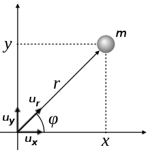
From the previous figure, and defining the velocities in $v_x$ and $v_y$ we obtain:

to get finally

Leap-frog Integration

The leap-frog scheme is an integration method inteded to solve differential equations associated to physical problems with implicit conservations laws (e.g. mechanical problems where the total energy is conserved). For this, suppose a problem of the form:

The leap-frog scheme gives the approximate solution through the next set of iterative expressions:

where $x_{i}$ denotes the position in the time $t_i = a + i\times \Delta t$, and $a$ is the initial time. The solution given by this procedure is less sensible to numerical losses of energy, unlike ordinary methods like Euler.

1. Solve the central force problem using the Euler's method given during class. Use the initial conditions compatible with the system Earth-Sun, i.e.

Integrate during five years using a timestep $\Delta t$ of 1 day ($86400\ s$). If you want, you can use a more convenient coordinate system in $days$ for time, $km$ for distance and $M_{\odot}$ for mass. (Remember you must change also the units of $G$). Plot the orbit $x(t)$ vs $y(t)$.

2. Repeat the same problem but using the leap-frog scheme. Plot the resulting orbit.

3. Calculate the total energy of the system:

for both integrators and compare them plotting $E_i$ vs $t_i$.

Questions:

• What can you conclude about the total energy of the systems when using the integrator schemes.

• what scheme deals better this problem?

#2) Gravitational Lensing

It is known that light rays are deflected when they pass near by a gravitational field, even since the newtonian theory, and that this deviation is proportional to the body mass which the light is interacting with and inversely proportional to the passing distance. Since it is common finding very massive structures in the universe and the measures that are done to study it involve photons, it makes sense to study what happens to a light source image when the rays get close to a grumpy object like a dark matter halo.

In order to study the light deflection in these cases, it will be used the simplest model, gravitational lens theory, where the len is a very massive object. A sketch of a typical system is shown in figure 1. The source plane is the light source or image that is going to be affected, $\eta$ is the distance from a image point to the line of sight and $\beta$ the subtended angle by the point. The lens plane corresponds to the mass that affects the light coming from the source, $\xi$ is the new image point distance to the line of sight, $\theta$ is the subtended angle by the new point position. Then, $\alpha$ is the deflection angle.

Since from observations $\theta$ is known, the problem to be solved per pixel is

but $\alpha$ also depends on $\theta$ besides the len halo properties. This would allow construct the real image from the distorted and magnified one.

<img src="./figures/lente.png";style="max-width:100%; width: 50%">

This equation can also be written in terms of distances

The solution to the lens equation is easier to get if it is assumed that the len is axially symmetric. In this case, the deflection angle takes the next form

The quantity $\Sigma$ is the surface mass density, i.e., the len's mass enclosed inside $\xi$ circle per area unit. It is important to notice that the direction of $\alpha$ is the same as $\xi$ and consequently $\eta$.

##Activities

The problem to be solved is the next: Given the stars positions of a galaxy find the image distorsion due to gravitational lensing.

For this, it is neccesary create a len toy (a real one should be constructed with a NFW profile) and solve the equation (2) to find $\xi$ given a point position of the source("star") $\eta$.

**1.(10$%$)** Create len toy: Generate a distribution (uniform or more concentrated on the center) of points of order size of 1000$pc$. This can be done generating a grid from x and y, where these arrays vary from 0 to the length. The total mass of the len must be $1e10M_{\odot}$, i.e., the magnitude order of mass of dark matter halo. Every point should have the same mass, and the masses sum must be the dark matter halo mass.

2.(10$%$) Load the stars positions of the galaxy. This is the image that is going to be distorted. It is recommended not using all of them, at least not until the code is already finished.

<img src="./figures/galaxia_2589.png";style="max-width:100%; width: 50%">

3.(40$%$) Solve the equation (2) using the len toy.

<img src="./figures/galaxia_lente_2589.png";style="max-width:100%; width: 50%">

**4. (20$%$)** Plot the distorted positions due to lensing, i.e., the x and y coordinates using$\xi$. You should obtain something like the figure 3.

**5.(10$%$)** Find the magnification,$\mu$, suffered for every point of the initial image(galaxy) finding the surface density,$\kappa$

to calculate $\kappa$ remember $\xi$ is the new position of every image point. Make a plot of $\xi$ vs $\mu$.

Since the equation 2 does not necessarily has a solution, it is recommended use the next $\textbf{magnitud order}$ for the system you are going to choose

*a) Distance to the source: 1e9pc

*b) Distance to the len, approximately the half the distance to the source

The constant values $G = 4.302\times 10^{-3}$ pc $M_{\odot}^{-1}$ $(km/s)^2$ and $c = 3e6$ km/s can be used.

The positions in the galaxy.dat are x and y in pc.

For every integration it can be used composite simpson rule(10$%$) , the scipy.integrate.quad is recommended for you to test the integration results.

**Hint ** The initial angle for every point in the image is the same that in the distorted image.

BONUS (+0.5 in theoretical test) Make a map with the magnification obtained using the positions $\xi$ of the image distorted. For this, suppose that all initial points have the same brightness.