SPH-simulation.ipynb

Kernel: Unknown Kernel

Task 2

This homework is an activity intended to practice the basic concepts of python and some of the functions offered by NumPy and Matplotlib.

Due to: May 17

Gas in cosmological simulations

For this task we are going to use a dataset of gas particles of a cosmological simulation. To do so, the cosmological code GADGET2 was used, implementing the hydrodynamical scheme SPH (Smoothed Particle Hydrodynaics). This cosmological simulation is consistent with the WMAP7 cosmology, and it has a comoving lenght of $20\ h^{-1}Mpc$ per side (a cubic box), with a resolution of $64^3=262144$ particles of gas.

The information of the gas particles can be downloaded from here. The order of the columns is:

1. ID of each particle.

2. X coordinate [$pc$ units].

3. Y coordinate [$pc$ units].

4. Z coordinate [$pc$ units].

5. X velocity component [$km/s$ units].

6. Y velocity component [$km/s$ units].

7. Z velocity component [$km/s$ units].

8. Mass of each particle. Same for all [$10^{10} M_{\odot}$ units].

9. Internal Energy.

10. Density.

11. Pressure.

12. Temperature.

13. Redshift.

14. Cosmological time [units in age of the universe].

Phase diagram of the gas

Using preferably ipython notebooks, perform the next activities:

• Load the previous dataset for the gas particles of the simulation.

• Normalize the density in order to obtain the density contrast. To do so, divide the column of densities by the value:

  $$\rho_{mean} = 278.458477853\ \Omega_b \times 10^{-10}\ M_{\odot}/kpc^3$$

  where $\Omega_b = 0.046$ is the density parameter of baryonic matter. Obtaining $\delta = \rho/\rho_{mean}$

• Using the function histogram2d of NumPy and the function imshow of Matplotlib, compute the phase diagram Density-Temperature-Pressure. You should obtain something like:

  

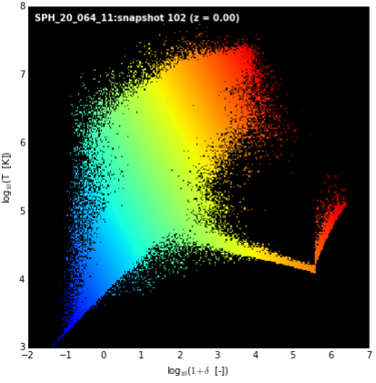
  Note that the 2D histogram is calculated over the $\log_{10}$ of each property.

Spatial distribution

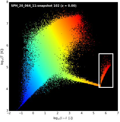
Gas particles inside dark matter halos exhibit a characteristic profile (white region in the next figure), being possible to extract those particles just by looking at the phase diagram.

• Make a 3D scatter plot of all the gas particles of the simulation. You shoud obtain something like this:

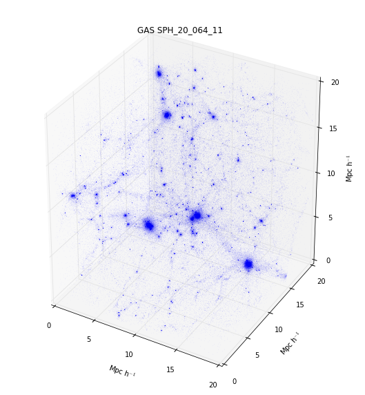
• Using the ranges $5.5 < \log_{10}(1+\delta) < 6.5$ and $4 < \log_{10}(T) < 5.5$ and the masking functions (e.g. X[X>5]), extract the coordinates $(x,y,z)$ of the gas particles satisfying both conditions. Then, in the same windows, make a 3D scatter plot of these particles (use a different color).

Tip: you can find a relatively complete example of the usage of 2D histograms in this notebook.

How to plot a 3D scatter

For making a 3D scatter, it is necessary to import the package Axes 3D in order to activate the 3D plotting.

%pylab inline
import matplotlib.pyplot as plt
from mpl_toolkits.mplot3d import Axes3D
#Activating 3D plotting
fig = plt.figure( figsize = (8,8) )
ax = fig.add_subplot(111, projection='3d')
X = [1,2,3,2,1,3,2,1]
Y = [3,2,1,3,2,1,3,2]
Z = [1,3,2,1,2,3,1,2]
ax.scatter( X, Y, Z )

Welcome to pylab, a matplotlib-based Python environment [backend: module://IPython.zmq.pylab.backend_inline].
For more information, type 'help(pylab)'.

<mpl_toolkits.mplot3d.art3d.Patch3DCollection at 0x3269310>

---