first_notebook.ipynb

Kernel: Unknown Kernel

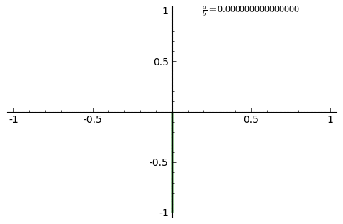
Lissajous curves

Lissajous curves are a family of parametric two-dimensional curves normally obtained when solving multi-harmonic systems, like a mass-spring systems with two springs in each axis (x and y) or some circuit systems. The figures are described with the following equations:

$$x(t) = A\sin(a t +\delta)$$$$y(t) = B\sin(b t)$$

where $A$ and $B$ are the amplitudes along each axis, $a$ and $b$ the angular frequencies and $\delta$ the relative phase.

#This line is always necessary when you use matplotlib in a notebook, otherwise the figures will not appear.
%pylab inline
import matplotlib.pyplot as plt
import numpy as np

Welcome to pylab, a matplotlib-based Python environment [backend: module://IPython.zmq.pylab.backend_inline].
For more information, type 'help(pylab)'.

Plotting some curves

#Solutions
def Lissajous( t, A=1.0, B=1.0, a=1.0, b=1.0, delta=0.0 ):
    x = A*np.sin(a*t+delta)
    y = B*np.sin(b*t)
    return x, y

#Parameters to be sampled--------------------
#delta
Ndelta = 4   #Number of delta parameters
Delta = np.linspace(0,np.pi,Ndelta)
#Ratio c=a/b
Nratio = 6  #Number of c parameters
C = np.linspace(0,1,Nratio)
#Time array
T = np.linspace(0,40,1000)

#Initializing plotting environment
plt.figure( figsize=(4*Ndelta, 4*Nratio) )
plt.subplot( Nratio, Ndelta, 1 )
plt.plot()
#Sweeping all figures
for i in xrange( Ndelta ):
    for j in xrange( Nratio ):
        #Creating a subfigure with the current delta and ratio c
        plt.subplot( Nratio, Ndelta, j*Ndelta+i+1 )
        #Plotting this Lissajous curve
        X, Y = Lissajous( T, b=C[j], delta=Delta[i] )
        plt.title( "$\delta=$%1.2f\t$a/b=$%1.2f"%(Delta[i],C[j]) )
        plt.plot( X, Y, linewidth=2 )

References

• http://en.wikipedia.org/wiki/Lissajous_curve