Task 9

This homework is an activity intended to apply the Euler's scheme for integrating differential equations. Besides, it is introduced a new scheme that conserves the energy of the system, i.e., the Leap-frog scheme.

Due to: Mar 8

Central Force Problem

The classic two-body problem with central force can be considerable simplified if one of the bodies has a mass much greater than the other one. In this case, the position of the most massive body (with mass $M$ ) will coincide with the center of mass of the system, and thus it is only interesting to find the position of the less massive body (with mass $m$ ) regarding the center of mass. The equation of motion for the body $m$ is then:

m\frac{d^2}{dt^2}\vec{r}(t) = F(r)\hat{u}_r

where $\vec{r}$ is the position of $m$ and $\hat{u}_r$ is a unitary vector pointing toward the origin of the central force. A very special case of this type of problems is the gravitation of a small body around a massive one, e.g. the earth-sun system, the moon-earth system, etc. For this case, $F(r)$ is replaced by the gravitational force, yielding:

m\frac{d^2}{dt^2}\vec{r}(t) = -G\frac{mM}{r^2}\hat{u}_r

For a central force problem is always possible to demonstrate that the complete movement will be constrained over a plane, so a suitable choice of coordinates will reduce the position to $\vec{r} = (x, y)$ and the previous equation yields:

\frac{d^2}{dt^2}x(t) = -G\frac{M}{r^2}\hat{u}_r\cdot \hat{u}_x

\frac{d^2}{dt^2}y(t) = -G\frac{M}{r^2}\hat{u}_r\cdot \hat{u}_y

where $\hat{u}_x$ and $\hat{u}_y$ are unitary vectors of the cartesian system. Note this set of equations does not depend on the mass of the small body.

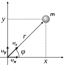
From the previous figure, and defining the velocities in $v_x$ and $v_y$ we obtain:

\hat{u}_r\cdot \hat{u}_x = \cos(\varphi) = \frac{x}{r}

\hat{u}_r\cdot \hat{u}_y = \sin(\varphi) = \frac{y}{r}

to get finally

\frac{d}{dt}v_x(t) = -G\frac{M}{r^3}x

\frac{d}{dt}x(t) = v_x(t)

\frac{d}{dt}v_y(t) = -G\frac{M}{r^3}y

\frac{d}{dt}y(t) = v_y(t)

Leap-frog Integration

The leap-frog scheme is an integration method inteded to solve differential equations associated to physical problems with implicit conservations laws (e.g. mechanical problems where the total energy is conserved). For this, suppose a problem of the form:

\frac{d}{dt}x(t) = v(t)

\frac{d}{dt}v(t) = F(x)

The leap-frog scheme gives the approximate solution through the next set of iterative expressions:

x_{i+1} = x_i + v_i\Delta t + \frac{1}{2}F(x_i)\Delta t^2

v_{i+1} = v_i + \frac{1}{2}[F(x_i)+F(x_{i+1})]\Delta t

where $x_{i}$ denotes the position in the time $t_i = a + i\times \Delta t$ , and $a$ is the initial time. The solution given by this procedure is less sensible to numerical losses of energy, unlike ordinary methods like Euler.

1. Solve the central force problem using the Euler's method given during class. Use the initial conditions compatible with the system Earth-Sun, i.e.

v_x(t=0) = 0

v_y(t=0) = 29780\ m/s

x(t=0) = 1.5\times 10^{11}\ m

y(t=0) = 0

M = 1.98855\times 10^{30}\ kg

Integrate during five years using a timestep $\Delta t$ of 1 day ( $86400\ s$ ). If you want, you can use a more convenient coordinate system in $days$ for time, $km$ for distance and $M_{\odot}$ for mass. (Remember you must change also the units of $G$ ). Plot the orbit $x(t)$ vs $y(t)$ .

2. Repeat the same problem but using the leap-frog scheme. Plot the resulting orbit.

3. Calculate the total energy of the system:

E_i = \frac{1}{2}(v_{xi}^2+v_{yi}^2) - G\frac{M}{r_i}\ \ \ \mbox{with}\ \ \ r_i = \sqrt{ x_{i}^2 + y_{i}^2 }

for both integrators and compare them plotting $E_i$ vs $t_i$ .

Questions:

What can you conclude about the total energy of the systems when using the integrator schemes.
what scheme deals better this problem?

Task 9

Central Force Problem

Leap-frog Integration

Product

Resources

Company