Test 1 - Computational Activity

This activity represents $50\%$ of the test 1. Each student must provide an ipython notebook with the solution of the proposed problems, along with all the performed procedures and related codes, as well as the obtained results.

Due to: Friday Jan 23, Midnight

Cooling Functions of Low-Density Astrophysical Plasmas

A plasma gas is a state of matter where atoms and/or molecules are so hot, that they reach the ionization threshold through thermal interactions (thermal ionization). This implies that the initial constituent particles (atoms and/or molecules) are broken up into positively charged ions and negatively charged electrons. As these singles constituents are not longer coupled, strong electrical and magnetic currents are generated, thus implying they are strongly influenced by electromagnetic interactions, unlike ordinary neutral matter.

Plasma physics is a mainstream topic in current astrophysics as almost all the baryonic matter in the universe is in this state. From solar and stellar physics, interplanetary, interstellar and intergalactic medium, active galactic nuclei up to large-scale structure formation are influenced by plasma processes.

In this activity we will investigate cooling functions $\Lambda(T)$ of a plasma slab under equilibrium conditions over a range of metallicities (fraction of elements heavier than Hydrogen and Helium) and temperatures ($10^4-10^{8.5}\ K$).

Cooling function: it is defined as the bolometric power emitted as thermal radiation by the plasma and normalized by the total emission, all as a function of the temperature. It is very important for estimating evolution of several plasmas.

Activities

In this folder you can find a set of simulated data for plasmas of different metallicities ($\{+0.5, 0.0, -0.5, -1.0, -1.5, -2.0, -3.0, \mbox{nil} \}$), where $0.0$ means a solar metallicity, and nil a zero metallicity model (no elements heavier than H and He). The file ABOUT.dat explains the information of each column, however we are interested in Temperature $\log10(T)$ (Column 0) and the normalized cooling function $\log10[\Lambda_N(T)]$ (Column 5).

Plotting for different metallicities, the next figure is obtained:

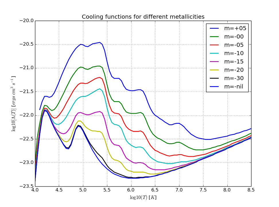
1. (10%) Reproduce the previous figure using the provided data.

2. (20%) Write a routine called CoolingFunction that, given any logarithmic temperature value $\log10(T)$ and a metallicity and using the provided data, interpolates (using either Linear or Lagrange interpolation) the value of the respective cooling function value.

3. (30%) Write a function called Temperature that, given any logarithmic value of the cooling function, metallicity value and a temperature guess value, calculate the respective temperature.

Note that this problem is the inverse problem of the previous item. You have to use the previous interpolation routine CoolingFunction, and using a find-root solver like Bisection or Fixed-Point iteration solve the next equation for the temperature

$\Lambda(T;m) = \Lambda_{0}$

$\Lambda(T;m) - \Lambda_{0} = 0$

where $\Lambda_{0}$ is the given value where you want to find evaluate the temperature. Remember, you have to provide a guess (or an interval) for the find-root solver.

4. (40%) Metallicity functions

A very interesting application of interpolation techniques is the estimation of Cooling functions in terms of metallicity. For this you need to perform a double interpolation procedure.

Given a fixed value of temperature $T_0$, you can evaluate all the Cooling functions for different metallicities, obtaining a set of values $\{m_i\}_i$ for the metallicities and $\{\Lambda_i(T_0)\}_i$ for the respective Cooling functions. This can be tought as tracing a vertical line in the previous figure passing through the given value $T_0$, and then taking all the intercepted values in the Cooling functions.

Make a figure where is plotted a set of Cooling functions ($y$-axis) as a function of the metallicity ($x$-axis), for the logarithmic temperatures of $\log10(T) = \{ 4.5, 5.0, 5.5, 6.0, 6.5, 7.0, 7.5, 8.0 \}$. This means, each curve corresponds with one of those temperature values.

Finally, write a routine called CoolingFunctionMetallicity that, given any metallicity value and any temperature value, calculates the respective Cooling function. Hint: for this routine you need the routine CoolingFunction of the second item for extracting the Cooling function values for different metallicities, obtaining $\{m_i\}_i$ and $\{\Lambda_i(T_0)\}_i$, then you have to perform another interpolation using these data, ant then evaluate at the given metallicity.

References

• Sutherland, R. S., and Dopita, M. A. "Cooling functions for low-density astrophysical plasmas." The Astrophysical Journal Supplement Series, 88 (1993): 253-327.

• http://ned.ipac.caltech.edu/level5/Sept08/Kaastra/Kaastra8.html

• Astrophysical Plasma

• Metallicity

• Data