Test 1 - Computational Activity

This activity represents $50\%$ of the test 1. Each student must provide an ipython notebook with the solution of the proposed problems, along with all the performed procedures and related codes, as well as the obtained results.

Due to: Monday Jun 15, Midnight

Internal Profiles of Rocky Planets

There is an increasing interest in studying rocky exoplanets due to the large amount of new discoveries, including recently earth-size planets. Modelling the internal properties of these planets is then prior to understanding them and to set posible theoretical constraints. In this activity we are going to use root finding and interpolation techniques to explore a set of simulated profiles of earth-size rocky planets produced using the software PLYNET.

Activities

Download these data. You will find a set of simulated planets with the same composition of the Earth (A iron core of Fe$_{08}$FeS$_{02}$ with a mass fraction of 0.325 and a mantle of pv_fmw with a mass fraction of 0.675, ocean layers are neglected). Each file contains 9 columns with tabulated properties of the respective planet, ordered as: normalized radial coordinate (0), radial coordinate in earth units (1), enclosed mass in earth mass units (2), density (3), pressure (4), gravity (5), potential (6), temperature (7) and a flag indicating the mantle or the core (8). Unless it is speficied, all units are in SI.

The objetive of this activity is to find possible mass scaling laws for earth-like planets. We are mainly interested in the density profiles.

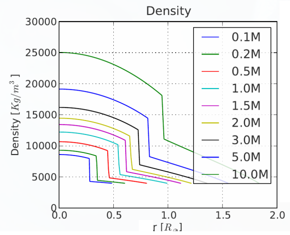
1. (10%) For all the planets provided, plot the radial coordinate (in earth units, column 1) vs the density profile, all in a same figure (reproduce the previous figure).

2. (20%) Write a routine called DensityFunction that, given a planetary mass (the name of the file to be opened) and a radius, returns the respective density. For this you can use either Linear interpolation or Lagrange interpolation. Take into account that for the Lagrange interpolator you have to adjust (decrease) the number of data in order to prevent numerical instabilities.

3. (30%) Write a function called Radius that, given any value of density and planetary mass (the name of the file to be opened) and a radial guess value, calculate the radius where that density is reached.

Note that this problem is the inverse problem of the previous item. You have to use the previous interpolation routine DensityFunction, and using a find-root solver like Bisection or Fixed-Point iteration solve the next equation for the radius

DensityFunction$(r;M_p) = \rho_{0}$

DensityFunction$(r;M_p) - \rho_{0} = 0$

where $\rho_{0}$ is the given value where you want to find the respective radius. Remember, you have to provide a guess (or an interval) for the find-root solver.

4. (40%) Center and mean density scaling laws

A very interesting application of interpolation techniques is the estimation of scaling laws in terms of central density and the average density. For this you need to perform a double interpolation procedure.

First, for the central density value, take the central value and the radial size of each planet and perform a Linear or Lagrange interpolation, plot the result. This result corresponds with the first scaling law.

For the second scaling law, you need to calculate the mean density of each planet, i.e. the total mass over the total volume. Once you obtain these values, you have to use the function Radius in order to find the respective radius where that mean density is reached inside the planet. Finally, write a new routine called MeanDensityLaw that with the previous values of mean density and radius of mean density, returns the mean density at any given radius. For this you need to perform an interpolation (Linear or Lagrange) again. Plot your results.

References

• PLYNET, Python Planetary Physics Pacakge. Bustamante, S. et al.