Test 2 - Computational Activity

This activity represents $50\%$ of the test 2. Each student must provide an ipython notebook with the solution of the proposed problems, along with all the performed procedures and related codes, as well as the obtained results.

Due to: Sunday Mar 1, Midnight

Integrated Spectrum of NGC 5947

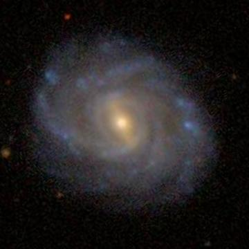
NGC 5947 is a barred spiral galaxy SBbc located in the Boötes constelation. For this activity, we are going to take an optical integral field spectrum (IFS) obtained by the CALIFA (The Calar Alto Legacy Integral Field Area) survey. These data come usually in the standard FITS format (you can download it from here). You can handle this format in python using for example the library PyFITS (installation).

However, we are going to use a set of ASCII files provided here, where the format spectra_i_j.dat is used for the spectrum of the i,j-th pixel of the image, and where $0\leq$i$\leq 71$ and $0\leq$j$\leq 77$, i.e. we have an image of $72\times 78$ pixels. Each file contains two columns, one with the wavelenght in units of Å, and the second with the respective flux in units of $1\times 10^{-16}$ erg s$^{-1}$ cm$^{-2}$ Å$^{-1}$.

For this activity, we intend to manipulate these spectra and integrate them numerically. For this purpose, we shall use the Composite Simpson's rule covered during class.

Activities

1. (10%) Create a routine that, given a set of points $\{x_i\}_i$ and $\{y_i\}_i$, computes the Composite Simpson's rule in the interval of the $x$ data.

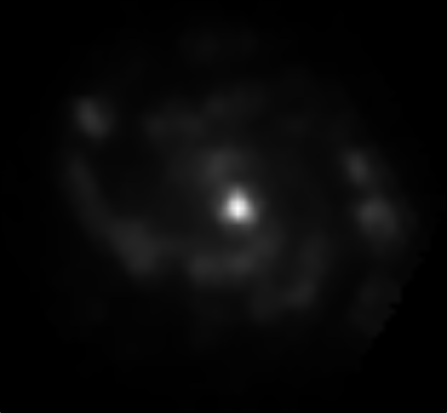
2. (10%) Integrated image of the galaxy: integrating the spectrum of each pixel over the optical range, we obtain the surface brightness of that pixel.

where $S^O_{ij}$ es the optical surface brightness of the i,j-th pixel, given in units of $1\times 10^{-16}$ erg s$^{-1}$ cm$^{-2}$, $I_{ij}$ the optical spectrum of that pixel, given in units of $1\times 10^{-16}$ erg s$^{-1}$ cm$^{-2}$ Å$^{-1}$, and $\lambda_0$ and $\lambda_1$ are the optical ranges, namely $\lambda_0 = 3749$ Å and $\lambda_1=7501$ Å.

Repeating this procedure for each pixel of the image, we obtain the optical surface brightness profile of the galaxy.

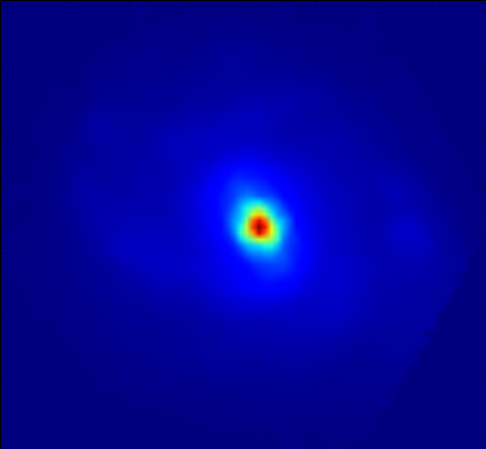
Using the previous routine, integrate the spectrum of each pixel, storing each result in a matrix. Finaly, using the function imshow of matplotlib, show the resulting image.

3. (20%) False coloured image: a very common colour model for representating images in a computer is based in three "beams" called components (RGB scheme), namely Red, Green and Blue components. For this activity we shall propose a simple and rough way to calculate these components for each pixel, provided the respective spectrum.

Associating the red component with the range $[ 5800$ Å, $7500$ Å$]$, the green component to $[ 4900$ Å, $5800$ Å$]$ and the blue component to $[ 4900$ Å, $3750$ Å$]$, we can integrate the spectrum of each pixel over these ranges, obtaining the respective surface brightness in each band.

Calculate the RGB indexes for each pixel of the galaxy $(C^r_{ij}, C^g_{ij}, C^b_{ij})$, then, normalize all the red components with the maxim value all over the galaxy. Repeat the same for green and blue components. This step must be done due to RGB indexes must range between $0$ and $1$.

Finally, using the same function imshow for showing a false colour of the galaxy. You should obtain something like:

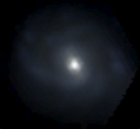
Tip: giving an array object with the components Galaxy[i,j,c], where $i$ and $j$ refer to the pixel position and $c=0,1,2$ refers to the R(0)-G(1)-B(0) indexes, imshow should give a real colour image.

4. (20%) H-alpha emission: the H$\alpha$ emission line is a spectral line of Hydrogen produced when a photon is emitted by an electron passing from the state of energy $n=3$ to the state $n=2$. The associated wavelenght is exactly $6562.8$ Å. For a spiral galaxy, this emission line normally appears in regions with high star formation rates like arms and bars.

For this activity, we are going to calculate the fully integrated spectra of the galaxy. From this, we can calculate the redshift of the galaxy, the total optical surface brightness and the emission map in the H$\alpha$ line.

Take all the spectra of the galaxy (each pixel) and average them in order to produce just one spectrum. This is the integrated spectrum of the galaxy. You should obtain something like:

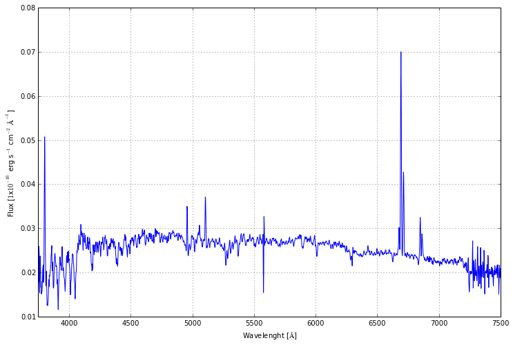
Integrate this spectrum over all the optical range, this result is the integrated surface brightness of all the galaxy.

The highest line in this spectrum corresponds with the H$\alpha$ emission line of all the galaxy. However, due to the expansion of the Universe, this line is shifted toward red. Locate this line of the spectrum $\lambda_{gal}$ and using the exact value of the H$\alpha$ line, calculate the redshift of this galaxy using the formula:

Once identified this line, integrate the spectrum of each pixel over the range $[\lambda_{gal}-\Delta \lambda, \lambda_{gal}+\Delta \lambda]$, with $\lambda_{gal}$ the H$\alpha$ line of the galaxy and $\Delta \lambda=5$ Å.

** Show the result using the imshow function. You should obtain something like:**

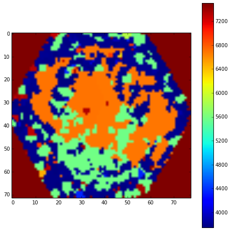
BONUS (+0.5 in theoretical test). Dominant emission line: although the core of the galaxy is far more dominating in the overall surface brightness, there are some regions where specific emission lines are dominant. Make a figure where the colour represents the dominant emission line for a given pixel. This is, take each pixel's spectrum, find the wavelength of maximum flux, and assign that value to that pixel. You should obtain something like:

N Coupled Linear Oscillators

In this activity we shall solve a set of N-coupled linear oscillators. This type of systems are very useful for modelling molecular dynamics and state solid systems. Let's suppose a set of $N$ mass $\{m_i\}_i$ coupled by $N$ strings of elastic constant $k_i$.

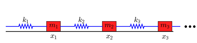
Defining the position $x_i(t)$ of the $i$th oscillator as its position of equilibrium (previous figure), each mass follows the next equation:

This is, the $i$th oscillator is coupled with the next one.

We then have to solve these equations in order to obtain the solutions $\{x_1(t),x_2(t),\cdots, x_N(t)\}$. In order to do this, we can define the matrix $\mathbf{M}$

then, the problem can be rewritten as

where $\mathbf{x}(t)$ is the vector of positions for all the oscillators.

If we can find a set of vectors $\mathbf{q}_k$ such that

where $\lambda_k$ is a eigenvalue of the matrix and $\mathbf{q}_k$ the respective eigenvector. There is then a matrix $\mathbf{A}$ such that

and

The initial problem becomes then:

The solution to this problem is given by

where $C_i$ and $\delta_i$ corresponds with the amplitude and the initial phase. The eigenvalues $\sqrt{\lambda_i}$ are then the natural frequencies of the problem.

Activities

1. (10%) Construct the matrix $\mathbf{M}$ of the problem for $N=10$ oscillators.

2. (15%) Using the function numpy.linalg.eig, calculate the eigenvalues $\{\lambda_i\}_i$ and the respective eigenvectors $\{\mathbf{u}_i\}_i$ of the matrix $\mathbf{M}$. Construct the diagonalising matrix giving by:

3. (15%) Using the found eigenvalues, plot the functions $q_i(t)$ for each normal mode of the oscillators. Then, using the matrix $\mathbf{A}$, find the solution to the problem in the original coordinate system. Plot in other figure all the solutions $x_i(t)$ for the oscillators.

Tip: use any set of initial conditions you want, i.e. the values $C_i$ and $\delta_i$ of the functions $q_i(t)$.