test3_20142.ipynb

Kernel: Unknown Kernel

Test 3 - Computational Activity

This activity represents $100\%$ of the test 1. Each student must provide an ipython notebook with the solution of the proposed problems, along with all the performed procedures and related codes, as well as the obtained results.

Due to: Tuesday Mar 23, Midnight

Henon-Heiles System

The Henon-Heiles system is a very used non-linear system of equations to illustrate the emergence of Hamiltonian Chaos by the mechanism of unfolding of torus. It was initially conceived by Michael Henon and Carl Heiles when working on the motion of stellar systems around a galactic centre where the motion is confined to a plane. The potential of the system is given by:

$$V(x,y) = \frac{1}{2}(x^2+y^2) + \lambda \left(x^2y - \frac{y^3}{3}\right)$$

The parameter $\lambda$ is usually taken as $\lambda = 1$. The Hamiltonian of the system is then given by:

$$\mathcal{H} = \frac{1}{2}(p_x^2+p_y^2) + \frac{1}{2}(x^2+y^2) + \lambda \left(x^2y - \frac{y^3}{3}\right)$$

Applying the canonical equations of motions, we obtain the next system:

$$\frac{dx}{dt} = \dot{x}(t) = p_x$$$$\frac{dp_x}{dt} = \dot{p}_x(t) = -x - 2\lambda x y$$$$\frac{dy}{dt} = \dot{y}(t) = p_y$$$$\frac{dp_y}{dt} = \dot{p}_y(t) = -y-\lambda(x^2 - y^2)$$

Instead of giving arbitrary initial conditions to this system, there is a more physical motivated way to do it. For a conservative mechanical system, the total energy of a system equals the Hamiltonian function:

$$e = \frac{1}{2}(p_x^2+p_y^2) + \frac{1}{2}(x^2+y^2) + \lambda \left(x^2y - \frac{y^3}{3}\right)$$

Due to the law of conservation of energy, $e$ must remains constant during the movement.

For choosing an appropriate set of initial conditions, we are going to use the next monte carlo technique:

• Set an arbitrary set of conditions $x = 0$, $y=y_0$, $p_y = p_{y0}$.

• Solve the equation of energy for $p_x^2$, obtaining:

  $$p_x^2 = 2e - p_y^2 - (x^2+y^2) - 2\lambda \left(x^2y - \frac{y^3}{3}\right)$$

• If the previous value of $p_x^2$ is negative, try again from step 1. If positive, take this as the initial value $p_{x0} = \sqrt{p_x^2}$.

• The obtained set $\{ x_0, y_0, p_{x0}, p_{y0} \}$ is compatible with the energy $e$ and can be used for solving the Henon-Heiles system.

Poincaré Map

A Poincaré map is a type of representation of a dynamical system where just a section of the phase space is studied. This is very useful when handling multidimensional phase spaces.

For the previous problem, suppose you have a solution given by $\{x(t), p_x(t), y(t), p_y(t)\}$. The Poincaré map associated to $y$ and $p_y$ can be constructed storing the points $\{y(t), p_y(t)\}$ everytime $x(t) = 0$. This can be though then as a plane cut of a four-dimensional phase space.

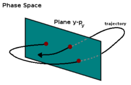
For the previous figure, the Poincaré map is the set of all the red points corresponding with the trajectory when crosses the plane $y-p_y$ (i.e. $x = 0$).

Activities

For this activity, we are going to use a RK4 integrator in order to solve the Henon-Heiles system. After that, we are going to construct Poincaré maps for initial conditions consistent with different energy values. For each energy value, it is possible to see the associated dynamics, seeing the emergence of chaotic regime (hamiltonian chaos or chaos in conservative systems) as we increase the energy.

1. (10%) Runge-Kutta 4

Write a routine called RK4-step(y,t,h) that, given the vector solutions y at certain time t, returns the solution for the next time interval t+h.

2. (10%) Dynamical Function

Write the dynamical function of the Henon-Heiles system. This is, a routine that given a vector with the variables of the system, it returns the corresponding derivatives for each one.

3. (5%) Parameter of the System

Define the next parameters of the system: $\lambda = 1$, $Y_{max}=0.5$, $P_{y,max}=0.5$, $\epsilon = 0.001$.

4. (10%) Henon-Heiles Potential

Plot, using the function contourf of the matplotlib library the function $V(x,y)$. For this you must construct a matrix where rows are associated to $x$ coordinates, while columns are to $y$ coordinates. You should obtain something like:

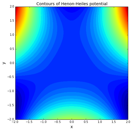
tip: you can use a double for cicle for constructing the matrix of the potential. This matrix can be then given as argument to the contourf function.

5. (35%) Poincaré Map Function

Define a routine called Poincare( energy, Ncond, tmax, h ) that, given a energy value (energy), the number of initial conditions to be integrated (Ncond), the maximum integration time (tmax) and the time step (h), calculates the Poincaré map of the system.

For this, you have to make first a for cicle over the number of initial conditions. It means something like:

#Poincare diagram
def Poincare( energy, Ncond, tmax, h ):
    #Specific solution
    ys = []
    pys = []
    #Finding initial conditions
    for n in xrange(Ncond):
        #... your code

where ys and pys are used to store the points of the Poincaré map, i.e., when the solution $x(t)=0$.

In numeral 3 you have defined two parameters, namely $Y_{max}$ and $P_{y,max}$. Using the monte carlo method exposed before, generate a random value y0 between $-Y_{max}$ and $Y_{max}$, then do the same for py0 between $-P_{y,max}$ and $P_{y,max}$. Set x0 = 0 and using the provided energy value to the Poincare routine and the equation for $p_x^2$, calculate that value. If $p_x^2<0$, the found set of initial conditions is not compatible with that energy. You must then repeat the process until you find a value $p_x^2>0$. Once there, make px0$=-\sqrt{p_x^2}$.

Using a second for, integrate the system over the time, until tmax, in time intervals of $h$. Inside that for, for every time, check the condition $|x(t)|<\epsilon$, i.e.

        #Integration
        i = 0
        for t in np.arange(0,tmax,h):
            y = [ X[i], PX[i], Y[i], PY[i] ]
            Xi, Pxi, Yi, Pyi = RK4_step( f, y, t, h )
            #Detecting a passing orbit through plane Y-Py
            if abs(Xi)<eps:
                ys.append( Yi )
                pys.append( Pyi )

If that is satisfied, store the respective value of Yi and Pyi, that is, the value of the coordinate $y$ and the momentum $p_y$ at that time.

You must repeat all of this for all the Ncond initial conditions. Finally plot, using a scatter diagram, the obtained array ys against pys. At this point, you have computed already the Poincaré map for the Henon-Heiles system.

6. (30%) Behaviour of Henon-Heiles System

Using the previous routine, study the behaviour of the Henon-Heiles system for the next energies:

$$e = \frac{1}{100},\ \ e = \frac{1}{12},\ \ e = \frac{1}{10},\ \ e = \frac{1}{8},\ \ e = \frac{1}{6}$$

tips: use a time step of $h=0.01$, a maxim integration time of $t_{max} = 400$ and a number of initial conditions $N_{cond} = 100$. You shoud obtain something like:

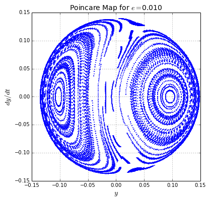
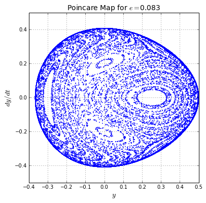
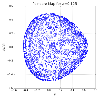
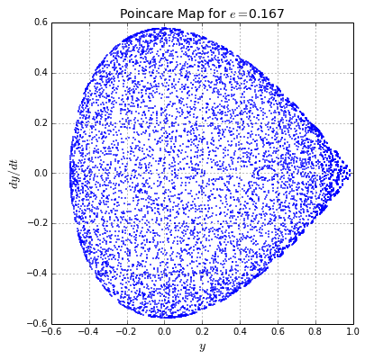
In this figures, it can be seen that, as the energy increases, the chaotic motion is more dominant. Oscillatory solutions (contrary to chaotic ones) are represented by circular orbits. In the first figure, for $e= 1/100$, all the orbits are oscillatory, while for the last figure, for $e=1/6$, orbits are chaotic as they do not present regular patrons.

References

• Hénon, M., Heiles, C. "The applicability of the third integral of motion: Some numerical experiments". The Astrophysical Journal 69: 73–79. (1964)

• Poincaré Map

---