GitHub Repository: restrepo/ComputationalMethods
Path: blob/master/material/linear-algebra-diagonalization.ipynb
⁹³⁴ views

Kernel: Python 3 (ipykernel)

Matrix diagonalization

Ortogonal matrices

\begin{align} x'=&x\cos\theta+y\sin\theta \nonumber\\ y'=&y\cos\theta-x\sin\theta\,. \end{align}

En forma matricial, la transformación del sistema de coordenas inicial al sistema de coordenados rotado por un ángulo $\theta$ está dado por $\begin{align} \begin{pmatrix} x'\\ y'\\ \end{pmatrix}= \begin{pmatrix} \cos\theta & \sin\theta\\ -\sin\theta& \cos\theta\\ \end{pmatrix} \begin{pmatrix} x\\ y\\ \end{pmatrix}. \end{align}$

Theorem 1

If $\boldsymbol{A}$ is Hermitic, e.g: $\begin{align} \boldsymbol{A}^\dagger =\boldsymbol{A}\,, \end{align}$ Then exists an unitary matrix $\boldsymbol{V}$ e.g: $\begin{align} \boldsymbol{V}^{\ -1}=\boldsymbol{V}^\dagger \,, \end{align}$ such that $\begin{equation} \boldsymbol{V}^\dagger\boldsymbol{A}\,\boldsymbol{V}=\boldsymbol{A}_{\text{diag}}\,, \end{equation}$ where $\boldsymbol{A}_{\text{diag}}=\operatorname{diag}(\lambda_1,\lambda_2,\ldots \lambda_n)$ is the diagonalized mass matrix.

Corollary 1

If $\boldsymbol{A}$ is symmetric, e.g: $\begin{align} \boldsymbol{A}^{\operatorname{T}} =\boldsymbol{A}\,, \end{align}$ Then exists an ortogonal matrix $\boldsymbol{V}$ , e.g: $\begin{align} \boldsymbol{V}^{-1}=\boldsymbol{V}^{\operatorname{T}} \,, \end{align}$ such that $\begin{equation} \boldsymbol{V}^{\operatorname{T}}\boldsymbol{A}\,\boldsymbol{V}=\boldsymbol{A}_{\text{diag}}\,, \end{equation}$ where $\boldsymbol{A}_{\text{diag}}=\operatorname{diag}(\lambda_1,\lambda_2,\ldots \lambda_n)$ is the diagonalized mass matrix.

Eigenvector problem

Note that each eigenvector, corresponding to each column of the matrix, is associated to each eigenvalue $\boldsymbol{V}=\begin{bmatrix} \boldsymbol{V}_1 \vdots \boldsymbol{V}_2\cdots \vdots \boldsymbol{V}_i \vdots \boldsymbol{V}_j\vdots\cdots \vdots \boldsymbol{V}_n \end{bmatrix}.$ where $\boldsymbol{V}_i$ is the $i$ -th column of the matrix $\boldsymbol{V}$ .

In this way, if we interchange the $i\leftrightarrow j$ columns of the diagonalization matrix $\boldsymbol{V}$ , the order of the eigenvalues also change $\begin{bmatrix} \boldsymbol{V}_1 \vdots \boldsymbol{V}_2\cdots \vdots \boldsymbol{V}_j \vdots \boldsymbol{V}_i\vdots\cdots \vdots \boldsymbol{V}_n \end{bmatrix}^\dagger \boldsymbol{A} \begin{bmatrix} \boldsymbol{V}_1 \vdots \boldsymbol{V}_2\cdots \vdots \boldsymbol{V}_j \vdots \boldsymbol{V}_i\vdots\cdots \vdots \boldsymbol{V}_n \end{bmatrix}=\operatorname{diag}(\lambda_1,\lambda_2,\ldots,\lambda_j,\lambda_i,\ldots \lambda_n).$ This property is very important because usually the diagonalizationn alghoritm gives not the desired ordering of the eigenvalues and eigenvectors. It is recommended to use the np.c_ method for the eigenvector reoirdering

However, the Theorem only guarantees existence. Tor really calculate the diagonalization matrix we must establish the eigenvector problem:

We can use the unitary propery to write $\begin{align} \boldsymbol{V}\boldsymbol{V}^\dagger\boldsymbol{A}\,\boldsymbol{V}=&\boldsymbol{V}\boldsymbol{A}_{\text{diag}}\\ \boldsymbol{A}\,\boldsymbol{V}=&\boldsymbol{V}\boldsymbol{A}_{\text{diag}}\,, \end{align}$ or $\boldsymbol{A}\begin{bmatrix} \boldsymbol{V}_1 \vdots \boldsymbol{V}_2\cdots \vdots \boldsymbol{V}_n \end{bmatrix} =\operatorname{diag}(\lambda_1,\lambda_2\ldots,\lambda_n)\begin{bmatrix} \boldsymbol{V}_1 \vdots \boldsymbol{V}_2\cdots \vdots \boldsymbol{V}_n \end{bmatrix}.$ Therefore, the eigenvalue equation is just: ParseError: KaTeX parse error: Expected & or \\ or \cr or \end at end of input: \begin{align} % \boldsymbol{A}\,\boldsymbol{V}_i=&\lambda_i\boldsymbol{V}_i \nonumber\\ \boldsymbol{A}\,\boldsymbol{V}_i-\lambda_i\boldsymbol{V}_i=&\boldsymbol{0} \nonumber\\ (\boldsymbol{A}-\lambda_i \,\boldsymbol{I})\boldsymbol{V}_i=&\boldsymbol{0}\,, %ParseError: KaTeX parse error: Expected 'EOF', got '\end' at position 2: \̲e̲n̲d̲{align} where $\boldsymbol{V}_i$ is the $i$ -th column of the matrix $\boldsymbol{V}$ , and $\boldsymbol{I}$ is the identity matrix.

To avoid the trivial solution $\boldsymbol{V}_i=\boldsymbol{0}$ , we require that $\boldsymbol{A}-\lambda_i\, \boldsymbol{I}$ does not have an inverse, or equivalently $\det( \boldsymbol{A}-\lambda_i\, \boldsymbol{I})=0\,.$

Example

From arXiv:2010.06458:

In the three flavor neutrino oscillation, the neutrino flavor states $\left|\nu_{\alpha}\right\rangle(\alpha=e, \mu, \tau)$ are linear superposition of mass eigenstates $\left|\nu_{j}\right\rangle(j=1,2,3):\left|\nu_{\alpha}\right\rangle=\Sigma_{j} U_{\alpha j}\left|\nu_{j}\right\rangle,$ where $U_{\alpha j}$ are the elements of the lepton mixing matrix known as PMNS (Pontecorvo-Maki-Nakagawa-Sakita) matrix such that $\left(\begin{array}{l} \left|\nu_{e}\right\rangle \\ \left|\nu_{\mu}\right\rangle \\ \left|\nu_{\tau}\right\rangle \end{array}\right)=\left(\begin{array}{lll} U_{e 1} & U_{e 2} & U_{e 3} \\ U_{\mu 1} & U_{\mu 2} & U_{\mu 3} \\ U_{\tau 1} & U_{\tau 2} & U_{\tau 3} \end{array}\right)\left(\begin{array}{l} \left|\nu_{1}\right\rangle \\ \left|\nu_{2}\right\rangle \\ \left|\nu_{3}\right\rangle \end{array}\right)$ The time evolution follows $\left|\nu_{\alpha}(t)\right\rangle=\Sigma_{j} e^{-i E_{j} t} U_{\alpha j}\left|\nu_{j}\right\rangle,$ where $E_{j}$ is the energy associated with the mass eigenstates $\left|\nu_{i}\right\rangle$ This is a superposition state.

The observables associated to the three neutrinos are the entries of the $3\times 3$ unitary matrix $\boldsymbol{U}=\begin{pmatrix}\boldsymbol{U}_1\vdots\boldsymbol{U}_2\vdots\boldsymbol{U}_3\end{pmatrix}$ , and the eigenvalues associated to each eigenvector $\boldsymbol{U}_1\to m_1$ , $\boldsymbol{U}_2\to m_2$ , $\boldsymbol{U}_3\to m_3$ . The normal ordering is $m_1<m_2<m_3$ . The unitary matrix can be parameterized in terms of three mixing angles, $\theta_{23}$ $\theta_{13}$ , $\theta_{12}$ , and a complex phase, $\delta_{\text{CP}}$ , such that $\boldsymbol{U}=\left(\begin{array}{ccc} 1 & 0 & 0 \\ 0 & c_{23} & s_{23} \\ 0 & -s_{23} & c_{23} \end{array}\right) \cdot\left(\begin{array}{ccc} c_{13} & 0 & s_{13} e^{-i \delta_{\mathrm{CP}}} \\ 0 & 1 & 0 \\ -s_{13} e^{i \delta_{\mathrm{CP}}} & 0 & c_{13} \end{array}\right) \cdot\left(\begin{array}{ccc} c_{12} & s_{12} & 0 \\ -s_{12} & c_{12} & 0 \\ 0 & 0 & 1 \end{array}\right),$ where $c_{i j} \equiv \cos \theta_{i j}$ and $s_{i j} \equiv \sin \theta_{i j}$ . Thus, we can write $\boldsymbol{U}$ as $\boldsymbol{U}=\left(\begin{array}{ccc}c_{12} c_{13} & s_{12} c_{13} & s_{13} e^{-i \delta_{\mathrm{CP}}} \\ -s_{12} c_{23}-c_{12} s_{13} s_{23} e^{i \delta_{\mathrm{CP}}} & c_{12} c_{23}-s_{12} s_{13} s_{23} e^{i \delta_{\mathrm{CP}}} & c_{13} s_{23} \\ s_{12} s_{23}-c_{12} s_{13} c_{23} e^{i \delta_{\mathrm{CP}}} & -c_{12} s_{23}-s_{12} s_{13} c_{23} e^{i \delta_{\mathrm{CP}}} & c_{13} c_{23}\end{array}\right)$ so that $\boldsymbol{U}_1=\begin{pmatrix}U_{e1}\\ U_{\mu 1}\\ U_{\tau 1}\end{pmatrix}=\begin{pmatrix} c_{12} c_{13} \\ -s_{12} c_{23}-c_{12} s_{13} s_{23} e^{i \delta_{\mathrm{CP}}} \\ s_{12} s_{23}-c_{12} s_{13} c_{23} e^{i \delta_{\mathrm{CP}}} \end{pmatrix},\qquad \boldsymbol{U}_2=\begin{pmatrix}U_{e2}\\ U_{\mu 2}\\ U_{\tau 2}\end{pmatrix}=\begin{pmatrix} s_{12} c_{13} \\ c_{12} c_{23}-s_{12} s_{13} s_{23} e^{i \delta_{\mathrm{CP}}} \\ -c_{12} s_{23}-s_{12} s_{13} c_{23} e^{i \delta_{\mathrm{CP}}} \end{pmatrix},\qquad \boldsymbol{U}_3=\begin{pmatrix}U_{e3}\\ U_{\mu 3}\\ U_{\tau 3}\end{pmatrix}=\begin{pmatrix} s_{13} e^{-i \delta_{\mathrm{CP}}} \\ c_{13} s_{23} \\ c_{13} c_{23} \end{pmatrix}$

After decades of experimental efforts with thousands of millions of dollars in investment and two recent Nobel prizes, most of the parameters are already measured (see PDG22020 ):

where $\Delta m^2_{ij}=m^2_i-m^2_j$ is the squared mass difference between eigenvalues $i$ and $j$ ; and $\text{eV}$ is really $\text{eV}/c^2$ where $c$ is the speed of light in vacuum in natural units with $c=1$ , and $1\ \text{eV}=1.602\,176\,6208(98)\times 10^{-19}\ \text{J}$ .

To a better measurement of $\delta_{CP}$ for example, a new large experiment called DUNE, and with a cost of around $$1\,500$ million of dollars, is in construction in the United States

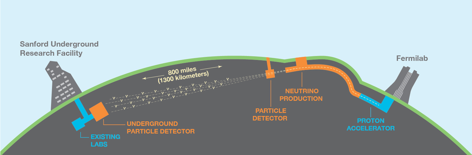
Theorem 2: Singular value decomposition (SVD)

See SVD (where the Hermetique-conjugate is denoted with "*" instead that with "")

A general complex matrix $\boldsymbol{A}$ can be diagonalized by a bi-diagonal transformation such that $\begin{equation} \boldsymbol{V}^\dagger\boldsymbol{A}\,\boldsymbol{U}=\boldsymbol{A}_{\text{diag}}\,, \end{equation}$ where $\boldsymbol{A}_{\text{diag}}=\operatorname{diag}(\lambda_1,\lambda_2,\ldots \lambda_n)$ is the diagonalized mass matrix.

Demostration

\begin{align} \boldsymbol{A}_{\text{diag}}=&\boldsymbol{V}^\dagger\boldsymbol{A}\,\boldsymbol{U}\\ \boldsymbol{A}_{\text{diag}}\boldsymbol{A}_{\text{diag}}^\dagger=&\boldsymbol{V}^\dagger\boldsymbol{A}\,\boldsymbol{U} \left(\boldsymbol{V}^\dagger\boldsymbol{A}\,\boldsymbol{U}\right)^\dagger\\ =&\boldsymbol{V}^\dagger\boldsymbol{A}\,\boldsymbol{U} \left( \boldsymbol{U}^\dagger \boldsymbol{A}^\dagger\,\boldsymbol{V}\right)\\ =&\boldsymbol{V}^\dagger \left( \boldsymbol{A} \boldsymbol{A}^\dagger\,\right) \boldsymbol{V}\,.\\ \end{align}

Since $\boldsymbol{A} \boldsymbol{A}^\dagger$ is hermitic and $\boldsymbol{A} \boldsymbol{A}^\dagger$ is diagonal, then in fact there exists an unitary matrix $\boldsymbol{V}$ . Similarly there exists an unitary matrix $\boldsymbol{U}$ which diagonalizes $\boldsymbol{A}^\dagger \boldsymbol{A}$

Scipy implementation

The implementation in scipy is based in the inverted relation $\begin{align} \boldsymbol{V}^\dagger\boldsymbol{A}\,\boldsymbol{U}=&\boldsymbol{A}_{\text{diag}}\\ \boldsymbol{V}\boldsymbol{V}^\dagger\boldsymbol{A}\,\boldsymbol{U}\boldsymbol{U}^\dagger=&\boldsymbol{V}\boldsymbol{A}_{\text{diag}}\boldsymbol{U}^\dagger\\ \boldsymbol{A}=&\boldsymbol{V}\boldsymbol{A}_{\text{diag}}\boldsymbol{U}^\dagger\,. \end{align}$

The implementation is trough the module scipy.linalg.svd:

V,Adiag,Udagger=linalg.svd(A)

Eigenvectors and eigenvalues

If we make $\boldsymbol{U}=[\boldsymbol{U}_1\vdots\boldsymbol{U}_2\vdots\cdots\vdots\boldsymbol{U}_n], \qquad \boldsymbol{V}=[\boldsymbol{V}_1\vdots\boldsymbol{V}_2\vdots\cdots\vdots\boldsymbol{V}_n]$

We know that there exists a bi-diagonal transformación such that ParseError: KaTeX parse error: Expected & or \\ or \cr or \end at end of input: …gin{equation} % \boldsymbol{A}\,\boldsymbol{U}=\boldsymbol{V}\boldsymbol{A}_{\text{diag}} \end{equation}$$ ParseError: KaTeX parse error: Expected & or \\ or \cr or \end at end of input: …ldsymbol{V}_i % \end{equation}$$ not sum upon $i$ . Here

$\lambda_i$ are called eigenvalues
$V_i$ and $U_i$ are the eigenvectors

We can use this to check the proper order of the eigenvalues

Transformation of a linear system

We start again with the matrix equation, capitol bold letters denotes matrices $\begin{equation} \boldsymbol{A}\boldsymbol{X}=\boldsymbol{B}\,, \end{equation}$ where $\boldsymbol{A}$ is an $n \times n$ matrix.

We know that there exists a bi-diagonal transformación such that $\begin{equation} \boldsymbol{V}^\dagger\boldsymbol{A}\,\boldsymbol{U}=\boldsymbol{A}_{\text{diag}} \end{equation}$ So, by doing standard operations we have $\begin{align} \boldsymbol{V}^\dagger \boldsymbol{A} \boldsymbol{U} \boldsymbol{U}^\dagger \boldsymbol{X}=& \boldsymbol{V}^\dagger \boldsymbol{B}\\ \left( \boldsymbol{V}^\dagger \boldsymbol{A} \boldsymbol{U} \right) \left( \boldsymbol{U}^\dagger \boldsymbol{X}\right)=& \boldsymbol{V}^\dagger \boldsymbol{B}\\ \boldsymbol{A}_{\text{diag}} \boldsymbol{X}'=&\boldsymbol{B}'\,, \end{align}$ where $\begin{align} \boldsymbol{X}'=& \boldsymbol{U}^\dagger \boldsymbol{X}\,, & \boldsymbol{B}'=& \boldsymbol{V}^\dagger \boldsymbol{B}\,, \end{align}$ or $\begin{align} \boldsymbol{X}=& \boldsymbol{U}\boldsymbol{X}'\,, & \boldsymbol{B}=& \boldsymbol{V}\boldsymbol{B}'\,. \end{align}$

If $\boldsymbol{A}_{\text{diag}}=\operatorname{diag}(\lambda_1,\lambda_2,\ldots \lambda_n)$ , $\boldsymbol{X}=\begin{pmatrix}x_1 & x_2 &\cdots & x_n\end{pmatrix}^{\operatorname{T}}$ and $\boldsymbol{B}=\begin{pmatrix}b_1& b_2 &\cdots & b_n\end{pmatrix}^{\operatorname{T}}$ , the solution of the system is given by $\begin{equation} \lambda_i x'_i=b_i'\,. \end{equation}$

Note that $\begin{align} \boldsymbol{X}'=&\boldsymbol{A}_{\text{diag}}^{-1}\boldsymbol{B}'\,, \end{align}$ and the final solution is $\begin{align} \boldsymbol{X}=&U \boldsymbol{X}'\\ =&U\boldsymbol{A}_{\text{diag}}^{-1}V^\dagger \boldsymbol{B}\,, \end{align}$ Therefore $\boldsymbol{A}^{-1}=U\boldsymbol{A}_{\text{diag}}^{-1}V^\dagger$

Example

A suitable way to introduce this method is applying it to some basic problem. To do so, let's take the result of the Example 1:

\begin{bmatrix} 5 & -4 & 0 \\ -4 & 7 & -3 \\ 0 & -3 & 5 \end{bmatrix} \begin{bmatrix} x_{1} \\ x_{2} \\ x_{3} \end{bmatrix} = \begin{bmatrix} 1 \\ 0 \\ -2 \end{bmatrix}

As the matrix is symmetric $\boldsymbol{U}=\boldsymbol{V}$ and $\boldsymbol{V}^\dagger=\boldsymbol{V}^{\operatorname{T}}$

In [1]:

import numpy as np

In [2]:

M1=np.array([[5,-4,0],
             [-4,7,-3],
             [0,-3,5]])

In [3]:

A=M1
A

Out[3]:

array([[ 5, -4,  0],
       [-4,  7, -3],
       [ 0, -3,  5]])

Check if all eigenvalues are different from zero:

In [4]:

np.linalg.det(A)

Out[4]:

49.99999999999999

In [5]:

B=np.c_[ [1,0,-2]  ]
B

Out[5]:

array([[ 1],
       [ 0],
       [-2]])

Also as

B=np.array([[1],[0],[-2]])
#or
B=np.reshape(  [1,0,-2],(3,1) )

Theorem 1 in `numpy`

WARNING: Only works for Hermitic matrices!

In [6]:

λ,V=np.linalg.eig( A )

In [7]:

A_diag=np.diag(λ)
A_diag

Out[7]:

array([[11.09901951,  0.        ,  0.        ],
       [ 0.        ,  0.90098049,  0.        ],
       [ 0.        ,  0.        ,  5.        ]])

In [8]:

Out[8]:

array([[-5.07191124e-01, -6.18673713e-01, -6.00000000e-01],
       [ 7.73342141e-01, -6.33988906e-01,  1.91548674e-16],
       [-3.80393343e-01, -4.64005285e-01,  8.00000000e-01]])

In [9]:

(V@V.transpose()).round(15).astype(int)

Out[9]:

array([[1, 0, 0],
       [0, 1, 0],
       [0, 0, 1]])

We first check the proper order of the diagonalization

In [10]:

(V.transpose()@A@V).round(14)

Out[10]:

array([[11.09901951,  0.        ,  0.        ],
       [ 0.        ,  0.90098049,  0.        ],
       [ 0.        ,  0.        ,  5.        ]])

In [11]:

(V.transpose().dot(A)).dot(V).round(14)

Out[11]:

array([[11.09901951,  0.        ,  0.        ],
       [ 0.        ,  0.90098049,  0.        ],
       [ 0.        ,  0.        ,  5.        ]])

Since

In [12]:

Out[12]:

array([[-5.07191124e-01, -6.18673713e-01, -6.00000000e-01],
       [ 7.73342141e-01, -6.33988906e-01,  1.91548674e-16],
       [-3.80393343e-01, -4.64005285e-01,  8.00000000e-01]])

The final solution is:

In [13]:

A_diag_inv=np.diag(1/λ)
A_diag_inv

Out[13]:

array([[0.09009805, 0.        , 0.        ],
       [0.        , 1.10990195, 0.        ],
       [0.        , 0.        , 0.2       ]])

check with np.linalg.inv(A_diag)

In [16]:

X=V@A_diag_inv@V.transpose()@B
X

Out[16]:

array([[ 0.04],
       [-0.2 ],
       [-0.52]])

Activity: Usar np.lingalg.solve

In [17]:

np.linalg.solve(A,B)

Out[17]:

array([[ 0.04],
       [-0.2 ],
       [-0.52]])

We can now check some properties.

\begin{equation} \boldsymbol{V}^{\operatorname{T}}\boldsymbol{A}\,\boldsymbol{V}=\boldsymbol{A}_{\text{diag}}\,, \end{equation}

\begin{bmatrix} \boldsymbol{V}_1 \vdots \boldsymbol{V}_2\cdots \vdots \boldsymbol{V}_j \vdots \boldsymbol{V}_i\vdots\cdots \vdots \boldsymbol{V}_n \end{bmatrix}^\dagger \boldsymbol{A} \begin{bmatrix} \boldsymbol{V}_1 \vdots \boldsymbol{V}_2\cdots \vdots \boldsymbol{V}_j \vdots \boldsymbol{V}_i\vdots\cdots \vdots \boldsymbol{V}_n \end{bmatrix}=\operatorname{diag}(\lambda_1,\lambda_2,\ldots,\lambda_j,\lambda_i,\ldots \lambda_n).

For the case $3\times 3$

Obtain $\theta_{12}$ for $|\lambda_1|<|\lambda_2|<|\lambda_3|$ and, in the proper order $\boldsymbol{U}=\left(\begin{array}{ccc}c_{12} c_{13} & s_{12} c_{13} & s_{13} e^{-i \delta_{\mathrm{CP}}} \\ -s_{12} c_{23}-c_{12} s_{13} s_{23} e^{i \delta_{\mathrm{CP}}} & c_{12} c_{23}-s_{12} s_{13} s_{23} e^{i \delta_{\mathrm{CP}}} & c_{13} s_{23} \\ s_{12} s_{23}-c_{12} s_{13} c_{23} e^{i \delta_{\mathrm{CP}}} & -c_{12} s_{23}-s_{12} s_{13} c_{23} e^{i \delta_{\mathrm{CP}}} & c_{13} c_{23}\end{array}\right)$

In [35]:

import numpy as np
A=np.array( [[5,-4,0],
             [-4,7,-3],
             [0,-3,5]])

λ,V=np.linalg.eig( A )
A_diag=np.diag(λ)
λ

Out[35]:

array([11.09901951,  0.90098049,  5.        ])

In [36]:

Out[36]:

array([[-5.07191124e-01, -6.18673713e-01, -6.00000000e-01],
       [ 7.73342141e-01, -6.33988906e-01,  1.91548674e-16],
       [-3.80393343e-01, -4.64005285e-01,  8.00000000e-01]])

Extract the first eigenvector

In [37]:

np.c_[ V[: ,0] ]

Out[37]:

array([[-0.50719112],
       [ 0.77334214],
       [-0.38039334]])

associated with the eigenvalue

In [38]:

A_diag[0,0],λ[0]

Out[38]:

(11.099019513592784, 11.099019513592784)

In [39]:

V0=np.c_[ V[:,0] ]
V1=np.c_[ V[:,1] ]
V2=np.c_[ V[:,2] ]
display(V0)
display(V1)
V2

Out[39]:

array([[-0.50719112],
       [ 0.77334214],
       [-0.38039334]])

array([[-0.61867371],
       [-0.63398891],
       [-0.46400528]])

array([[-6.00000000e-01],
       [ 1.91548674e-16],
       [ 8.00000000e-01]])

Check: $A V_i=\lambda_i V_i$

Which means the eigenvalue associated to the "operator" $A$ acting on the eigenvector $V_1$

In [40]:

print(f'{A@V0} =\n{λ[0]*V0}')

Out[40]:

[[-5.62932419]
 [ 8.58333952]
 [-4.22199314]] =
[[-5.62932419]
 [ 8.58333952]
 [-4.22199314]]

In [41]:

print(f'{A@V1} =\n{λ[1]*V1}')

Out[41]:

[[-0.55741294]
 [-0.57121163]
 [-0.41805971]] =
[[-0.55741294]
 [-0.57121163]
 [-0.41805971]]

In [42]:

print(f'{(A@V2).round(14)} =\n{(λ[2]*V2).round(14)}')

Out[42]:

[[-3.]
 [ 0.]
 [ 4.]] =
[[-3.]
 [ 0.]
 [ 4.]]

The diagonalization matrix can be rebuild from the eigenvectors

In [43]:

Out[43]:

array([[-5.07191124e-01, -6.18673713e-01, -6.00000000e-01],
       [ 7.73342141e-01, -6.33988906e-01,  1.91548674e-16],
       [-3.80393343e-01, -4.64005285e-01,  8.00000000e-01]])

is rebuild with

In [44]:

V=np.c_[ V0,V1,V2]

or with: np.hstack((V0,V1,V2))

In [45]:

Out[45]:

array([[-5.07191124e-01, -6.18673713e-01, -6.00000000e-01],
       [ 7.73342141e-01, -6.33988906e-01,  1.91548674e-16],
       [-3.80393343e-01, -4.64005285e-01,  8.00000000e-01]])

In [46]:

( V.transpose()@A@V).round(14)

Out[46]:

array([[11.09901951,  0.        ,  0.        ],
       [ 0.        ,  0.90098049,  0.        ],
       [ 0.        ,  0.        ,  5.        ]])

Note that a sign of an egigenvalues can be changed:

In [47]:

V=np.c_[ V0,-V1,V2]

Eigenvector reordering

Activity: https://beta.deepnote.com/project/17b487c8-b092-4032-94f5-438ba4eeb1e9

We can use this to check the proper order of the eigenvalues.

The order of eigenvalues can now be changed by changing the order of the eigenvectors and redifining the diagonalization matrix. For example, from small to large.

Then the proper order in the eigenvalues can be obtained

In [49]:

U=np.c_[ V1,V2,V0]
( U.transpose()@A@U).round(14)

Out[49]:

array([[ 0.90098049,  0.        ,  0.        ],
       [ 0.        ,  5.        ,  0.        ],
       [ 0.        ,  0.        , 11.09901951]])

In [51]:

Out[51]:

array([[-6.18673713e-01, -6.00000000e-01, -5.07191124e-01],
       [-6.33988906e-01,  1.91548674e-16,  7.73342141e-01],
       [-4.64005285e-01,  8.00000000e-01, -3.80393343e-01]])

Once in the proper order, the mixing angles can be obtained $\boldsymbol{U}_1=\begin{pmatrix}U_{e1}\\ U_{\mu 1}\\ U_{\tau 1}\end{pmatrix}=\begin{pmatrix} c_{12} c_{13} \\ -s_{12} c_{23}-c_{12} s_{13} s_{23} e^{i \delta_{\mathrm{CP}}} \\ s_{12} s_{23}-c_{12} s_{13} c_{23} e^{i \delta_{\mathrm{CP}}} \end{pmatrix},\qquad \boldsymbol{U}_2=\begin{pmatrix}U_{e2}\\ U_{\mu 2}\\ U_{\tau 2}\end{pmatrix}=\begin{pmatrix} s_{12} c_{13} \\ c_{12} c_{23}-s_{12} s_{13} s_{23} e^{i \delta_{\mathrm{CP}}} \\ -c_{12} s_{23}-s_{12} s_{13} c_{23} e^{i \delta_{\mathrm{CP}}} \end{pmatrix},\qquad \boldsymbol{U}_3=\begin{pmatrix}U_{e3}\\ U_{\mu 3}\\ U_{\tau 3}\end{pmatrix}=\begin{pmatrix} s_{13} e^{-i \delta_{\mathrm{CP}}} \\ c_{13} s_{23} \\ c_{13} c_{23} \end{pmatrix},$ so that $\tan\theta_{12}=\frac{U_{e2}}{U_{e1}}$

In [52]:

θ_12=np.arctan( U[0,1]/U[0,0] )

In [53]:

θ_12, θ_12*180/np.pi

Out[53]:

(0.7700763823614476, 44.122126612013574)

Implementation of an algorithm for reordering

In [54]:

λ

Out[54]:

array([11.09901951,  0.90098049,  5.        ])

In [56]:

np.sort( np.abs(λ))

Out[56]:

array([ 0.90098049,  5.        , 11.09901951])

Returns the indices that would sort an array.

In [58]:

index=np.abs(λ).argsort()
index

Out[58]:

array([1, 2, 0])

can be implemented in general with a comprehension list

In [59]:

Out[59]:

array([[-5.07191124e-01,  6.18673713e-01, -6.00000000e-01],
       [ 7.73342141e-01,  6.33988906e-01,  1.91548674e-16],
       [-3.80393343e-01,  4.64005285e-01,  8.00000000e-01]])

For rebuild

In [60]:

np.c_[ tuple( [ np.c_[V[:,i]]    for i in range(3) ] ) ]

Out[60]:

array([[-5.07191124e-01,  6.18673713e-01, -6.00000000e-01],
       [ 7.73342141e-01,  6.33988906e-01,  1.91548674e-16],
       [-3.80393343e-01,  4.64005285e-01,  8.00000000e-01]])

And for reorder to index

In [62]:

U=np.c_[ tuple( [ np.c_[V[:,i]]    for i in np.abs(λ).argsort() ] ) ]
U

Out[62]:

array([[ 6.18673713e-01, -6.00000000e-01, -5.07191124e-01],
       [ 6.33988906e-01,  1.91548674e-16,  7.73342141e-01],
       [ 4.64005285e-01,  8.00000000e-01, -3.80393343e-01]])

or:

n=3
U=np.hstack( [ np.reshape( V[:,i], (n,1) ) for i in index   ] )

In [63]:

( U.transpose()@A@U).round(14)

Out[63]:

array([[ 0.90098049, -0.        , -0.        ],
       [-0.        ,  5.        ,  0.        ],
       [-0.        ,  0.        , 11.09901951]])

Implementation as function

In [64]:

def argeig(A):
    λ,V=np.linalg.eig(A)
    λ=np.array([λ[i] for i in np.abs(λ).argsort()])
    V=np.c_[ tuple( [ np.c_[V[:,i]] for i in np.abs(λ).argsort() ] ) ]
    return λ,V

In [65]:

λ,V=argeig(A)
λ,V

Out[65]:

(array([ 0.90098049,  5.        , 11.09901951]),
 array([[-5.07191124e-01, -6.18673713e-01, -6.00000000e-01],
        [ 7.73342141e-01, -6.33988906e-01,  1.91548674e-16],
        [-3.80393343e-01, -4.64005285e-01,  8.00000000e-01]]))

#1.
λ,V=argeig(A)
λ,V
Out[1]:
(array([ 0.90098049,  5.        , 11.09901951]),
 array([[-6.18673713e-01, -6.00000000e-01, -5.07191124e-01],
        [-6.33988906e-01,  1.91548674e-16,  7.73342141e-01],
        [-4.64005285e-01,  8.00000000e-01, -3.80393343e-01]]))

#2.
(  V.transpose()@A@V).round(14)
Out[1]:
array([[ 0.90098049,  0.        ,  0.        ],
       [ 0.        ,  5.        ,  0.        ],
       [ 0.        ,  0.        , 11.09901951]])

#3.
print( np.linalg.det(A- λ[0]*np.identity(3) ) )
print( np.linalg.det(A- λ[1]*np.identity(3) ) )
np.linalg.det(A- λ[2]*np.identity(3) )

Activity: Build a function that diagonalize symmetric matrices with the eigenvalues in increasing order in the eigenvalues as a replacement of np.linalg.eig

def argeig(A):
    l,V=np.linalg.eig(A)
    ....
    return argl, argV

General matrix

In [107]:

import numpy as np
from scipy import linalg

Example: Consider the following general real matrix without any specific symmetry

In [119]:

A=np.array([[ 6.666746440000001  , 3.1312125300000013],
            [-0.23343504999999923, 5.890289299999999 ]])

In this case we need to make the bidiogalization process of Theorem 2 with the Singular value decomposition (SVD) implemented in Scipy

In [120]:

V,diag,Udagger=linalg.svd(A)

In [121]:

U=Udagger.transpose().conjugate()

In [122]:

A_diag=(V.transpose().conjugate()@A@U).round(14)
A_diag

Out[122]:

array([[ 8., -0.],
       [ 0.,  5.]])

This is important to stablish that the eigenvectors are determined until ordering and permutations

In [123]:

Out[123]:

array([[-0.8660254, -0.5      ],
       [-0.5      ,  0.8660254]])

In [124]:

Out[124]:

array([[-0.70710678, -0.70710678],
       [-0.70710678,  0.70710678]])

For a general matrix they are just ortogonal matrices

In [125]:

(U.transpose()@U).round(14)

Out[125]:

array([[1., 0.],
       [0., 1.]])

We define below a $2\times 2$ orthogonal matrix:

In [126]:

def orthogonal(θ):
    return np.array( [[np.cos(θ) ,np.sin(θ)],
                      [-np.sin(θ),np.cos(θ)]]   )

In [127]:

π=np.pi
Vp=orthogonal(π/3)
Vp

Out[127]:

array([[ 0.5      ,  0.8660254],
       [-0.8660254,  0.5      ]])

Note that, for $V=[V_1\vdots V_2]$ , after

Interchange $V_1 \to V_2$ and $V_2 \to V_1$
$V \to -V$ ,

we get $V'$

In [128]:

Up=orthogonal(π/4)
Up

Out[128]:

array([[ 0.70710678,  0.70710678],
       [-0.70710678,  0.70710678]])

Note that after

Interchange $U_1 \to U_2$ and $U_2 \to U_1$
$U \to -U$ ,

we get $U'$ .

Since the required trasformations in $V$ and $U$ are the same, the Theorem 2 is unnafected, only the order in the eigenvalues change to the normal ordering. In Fact

In [130]:

A_diag=(Vp.transpose()@A@Up).round(8)
A_diag

Out[130]:

array([[ 5., -0.],
       [ 0.,  8.]])

Activity: https://beta.deepnote.com/project/17b487c8-b092-4032-94f5-438ba4eeb1e9

Activity: Solve the system $\boldsymbol{A} \boldsymbol{x}=\boldsymbol{B}$ for the previous $\boldsymbol{A}$ matrix and $\boldsymbol{B}=\begin{bmatrix} 1\\ -4\\ \end{bmatrix}$

Interpretations of Theorem 2

Single Diagonalization matrix

In Theorem 2 establishes a unique set of a matrices: $A$ with its eigenvalues matrix, $A_{\rm diag}$ , and their eigenvectors matrices $U$ and $V$ . However, for a fixed set of eigenvalues and eigenvectors we can have several possibilities of $A'$ matrices. For example, if we fix $U'=\boldsymbol{1}$ $\begin{equation} {V'}^\dagger \boldsymbol{A'}=\boldsymbol{A}_{\text{diag}}\,, \end{equation}$ so that $\begin{equation} \boldsymbol{A}'=V'\boldsymbol{A}_{\text{diag}} \end{equation}$

Therefore: Under this conditions, for a fixed set of eigenvalues and eigenvectors (associated to the matrix $V'$ ) there is a unique $A'$ matrix

Example Let $V'=U^{\operatorname{T}} V$ in the previous example. Find the matrix $A'$ which gives rise to the same eigenvalues

In [133]:

Adiag=np.array( [[5,0],
                 [0,8]] )

In [134]:

Vp=orthogonal(np.pi/4).transpose()@orthogonal(np.pi/3)
Vp

Out[134]:

array([[ 0.96592583,  0.25881905],
       [-0.25881905,  0.96592583]])

In [135]:

Ap=Vp@Adiag
Ap

Out[135]:

array([[ 4.82962913,  2.07055236],
       [-1.29409523,  7.72740661]])

In [136]:

(Vp.transpose()@Ap).round(14)

Out[136]:

array([[5., 0.],
       [0., 8.]])

Finally, we can use the full procedure of hermitic matrices to obtain the bidiagonal matrices $U,V$

Example: Diagonalize the matrix $A$ by using the Theorem 1 instead

In [137]:

A=np.array([[ 6.66674644,  3.13121253],
            [-0.23343505,  5.8902893 ]])

In [139]:

A@A.transpose()

Out[139]:

array([[54.25      , 16.88749537],
       [16.88749537, 34.74999996]])

In [140]:

A.transpose()@A

Out[140]:

array([[44.50000002, 19.50000001],
       [19.50000001, 44.49999995]])

→ is obtained with <ALT GR>+i or, similarly: ↓←

In [141]:

λ2,V=np.linalg.eig( A@A.transpose() )
print(λ2,'→',np.sqrt(λ2))
#V=np.c_[ -V[:,0],V[:,0]  ]
V

Out[141]:

[63.99999999 24.99999997] → [8. 5.]

array([[ 0.8660254, -0.5      ],
       [ 0.5      ,  0.8660254]])

In [142]:

λ2p,U=np.linalg.eig( A.transpose()@A  )
print(np.sqrt(λ2))
U

Out[142]:

[8. 5.]

array([[ 0.70710678, -0.70710678],
       [ 0.70710678,  0.70710678]])

In [143]:

(V.transpose()@A@U ).round(14)

Out[143]:

array([[ 8., -0.],
       [ 0.,  5.]])

Actividad: Make the algorithm of reordering for theorem 2

Mixed terms

Let: $\begin{align} X' = \begin{bmatrix} B \\ W \\ \end{bmatrix} \end{align}$

Consider the quadratic equation $\begin{align} X^{\prime\operatorname{T}} M X^\prime=& \begin{bmatrix} B & W \end{bmatrix} \begin{bmatrix} M_{11} & M_{12} \\ M_{12} & M_{22} \\ \end{bmatrix} \begin{bmatrix} B \\ W \\ \end{bmatrix}\\ =& \begin{bmatrix} B & W \end{bmatrix} \begin{bmatrix} M_{11}B + M_{12}W \\ M_{12}B + M_{22}W \\ \end{bmatrix}\\ =& B( M_{11}B + M_{12}W)+ W ( M_{12}B + M_{22}W )\\ =&M_{11} B^2 + 2M_{12} BW+ M_{22} W^2\,. \end{align}$ The quadratic equation is in terms of: $M_{11}$ , $M_{12}$ y $M_{22}$

We can simplify this expression if we change to a new basis $X=\begin{bmatrix} A\\ Z \end{bmatrix}$ in which $M$ is diagonal, in such a case the crossed term would disappear. The rotation from $X'\to X$ is defined by $\begin{align} X'= \begin{bmatrix} B\\ W \end{bmatrix}\equiv \begin{bmatrix} \cos\theta & \sin\theta\\ -\sin\theta & \cos\theta \end{bmatrix} \begin{bmatrix} A\\ Z \end{bmatrix}= V X \end{align}$ where $V$ is the rotation matrix $V=\begin{bmatrix} \cos\theta & \sin\theta\\ -\sin\theta & \cos\theta \end{bmatrix}.$ Therefore $\begin{align} X\equiv \begin{bmatrix} A\\ Z \end{bmatrix}=V^{\operatorname{T}} X' \to X^{\operatorname{T}}= X^{\prime\operatorname{T}} V\,, \end{align}$

In the new basis $\begin{align} X^{\prime\operatorname{T}} M X^\prime=&X^{\prime\operatorname{T}}V V^{\operatorname{T}} M V V^{\operatorname{T}} X^\prime\\ =&(X^{\prime\operatorname{T}}V) (V^{\operatorname{T}} M V) (V^{\operatorname{T}} X^\prime)\\ =& X^{\operatorname{T}} M_{\text{diag}} X \\ =& \lambda_1 A^2+\lambda_2 Z^2\,. \end{align}$

such that $|\lambda_1|\le|\lambda_2|$ , where $\begin{align} M_{\text{diag}}\equiv V^{\operatorname{T}} M V=\begin{bmatrix} \lambda_1 & 0 \\ 0 & \lambda_2 \\ \end{bmatrix}\,, \end{align}$

In this basis, the quadratic equation is in terms of eigenvalues and mixing angle, $\theta$ . Therefore, there are not longer mixed terms.

The diagonalization of quadratic equations can be straightforwardly generalized to $n$ -th degree equations in terms of $n\times n$ matrices

In [145]:

import numpy as np
g =0.64996
gp=0.35523
v=246.22046 #GeV

Example: Electroweak interactions

To understand the electromagnetic and weak fundamental interactions, the mathematical formulation need to be done in one basis where the photon field, denoted with a symbol $A$ , is still not well defined. Instead, the field $B$ , the precursor of $A$ , appears along with the weak field $W$ , the precursor of the electroweak field $Z$ . In the mathematical basis we have then $\begin{align} X' = \begin{bmatrix} B \\ W \\ \end{bmatrix}, \end{align}$ and there, the symmetric mass matrix is calculated as (Details here: PDF)

In [146]:

M=(v**2/4)*np.array([[gp**2,-g*gp],
                     [-g*gp, g**2]])

In [147]:

Out[147]:

array([[ 1912.52692086, -3499.32718938],
       [-3499.32718938,  6402.67629426]])

Checking that the determinant is zero

In [148]:

np.linalg.det(M).round(8)

Out[148]:

0.0

This imply that one egivanlue is zero

In [149]:

np.linalg.eigvals(M).round(12)

Out[149]:

array([   0.        , 8315.20321512])

which means that the matrix rank, the number of non-zero eigenvalues, is 1

In [150]:

np.linalg.matrix_rank(M)

Out[150]:

1

To make the change to the phyisical basis, $X=\begin{bmatrix} A\\ Z \end{bmatrix}$ through the rotation matrix $V=\begin{bmatrix} \cos\theta_W & \sin\theta_W\\ -\sin\theta_W & \cos\theta_W \end{bmatrix},$ the following transformation need to be established $\begin{align} X'= \begin{bmatrix} B\\ W \end{bmatrix}\equiv \begin{bmatrix} \cos\theta_W & \sin\theta_W\\ -\sin\theta_W & \cos\theta_W \end{bmatrix} \begin{bmatrix} A\\ Z \end{bmatrix}= V X\,, \end{align}$ such that $V$ is the diagonalization matrix of $M$

M_{\text{diag}}=V^{\operatorname{T}} M V

with the normal ordering: $|\lambda_1|\le|\lambda_2|$ , and

$V$ → Diagonalization matrix
$V$ → Ortogonal matrix
$V$ → Rotation matrix

To obtain the eigensystem, we use

In [152]:

λ,V=np.linalg.eig(M)

which in fact satisfy

In [153]:

( V.transpose()@M@V).round(12)

Out[153]:

array([[  -0.        ,    0.        ],
       [   0.        , 8315.20321512]])

Since the first (zero) eigenvalue is the one associated to $A$ , we can interpret directly the rotation matrix without changing the order of the eigenvectors

In [154]:

Out[154]:

array([[-0.87749437,  0.47958694],
       [-0.47958694, -0.87749437]])

Note that in fact, the absolute value of the first element of the first eigenvector is the larger one and corresponds to the component along the $B$ -axis.

Therefore

In [155]:

θ_W=np.arcsin( V[0,1] )
θ_W

Out[155]:

0.5001839211647364

The eigenvalue associated to $Z$ is

In [156]:

mZ=np.sqrt(λ[1])
mZ #GeV

Out[156]:

91.18773610041056

corresponding to the $Z$ mass in units of $\text{GeV}/c^2$ . As a reference, the proton mass is approximately $1\ \text{GeV}/c^2$

The physical observable associated to the weak mixing angle, $\theta_W$ , is (see PDF, along with the $Z^0$ boson mass, $m_Z$ )

In [157]:

np.sin(θ_W)**2

Out[157]:

0.23000362966286086

Corolary 1 Theorem II

For a unique unitary $n\times n$ matrix $\boldsymbol{V}$ and a set of unique of eigenvalues $\lambda_1,\lambda_2,\ldots\lambda_n$ there exists an infite set of mass matrices $\boldsymbol{A}$ , associated to the infinite sets of matrices $\boldsymbol{U}$ , such that $\boldsymbol{V}^\dagger\boldsymbol{A}\,\boldsymbol{U}=\boldsymbol{A}_{\text{diag}}\,,$ where $\boldsymbol{A}_{\text{diag}}=\operatorname{diag}(\lambda_1,\lambda_2,\ldots \lambda_n)$ is the diagonalized mass matrix. In particular, if $\boldsymbol{A}$ is hermitic then there is only one possibility for $\boldsymbol{U}=\boldsymbol{V}$ and therefore $\boldsymbol{A}$ is unique.

Corolary 2 Theorem II

An unique hermitic mass matrix, $\boldsymbol{A}$ , can be generated from an infinite set of arbitrary matrices $\boldsymbol{Y}$ , such that $\boldsymbol{A}=\boldsymbol{Y}^{\dagger}\boldsymbol{Y}$

Example: Neutrino mass matrix

Returning back to the neutrino mixing discussion, it is worth noticing that in the mathematical basis $N=\left(\begin{array}{l} \left|\nu_{e}\right\rangle \\ \left|\nu_{\mu}\right\rangle \\ \left|\nu_{\tau}\right\rangle \end{array}\right)$ the mass matrix, $\mathcal{M}_\nu$ is non-diagonal. However, if we assume that it is hermitic, then an unitary tranformation (rotation in the symmetric case), $\boldsymbol{U}$ ,can be defined to diagonal basis as $\left(\begin{array}{l} \left|\nu_{e}\right\rangle \\ \left|\nu_{\mu}\right\rangle \\ \left|\nu_{\tau}\right\rangle \end{array}\right)= \boldsymbol{U}\left(\begin{array}{l} \left|\nu_{1}\right\rangle \\ \left|\nu_{2}\right\rangle \\ \left|\nu_{3}\right\rangle \end{array}\right),$ which is identified as the diagonalization matrix $\boldsymbol{U}^\dagger \mathcal{M}_\nu \boldsymbol{U}=\operatorname{diag}(m_1,m_2,m_3).$

According to the corrolary there is a set of infinite matrices complatible with an unique $\boldsymbol{U}$ and the eigenvalues $m_1,m_2,m_3$

Casas-Ibarra parameterization

Consider a $n\times n$ symmetric matrix $A$ . We can assumme without lost of generality that this can be generated from a matrix $Y$ such that $A=Y^{\operatorname{T}}Y$ Theorem 1 gurantees that exists an ortogonal matrix $U$ such that $U^{\operatorname{T}} A U=U^{\operatorname{T}} Y^{\operatorname{T}}Y U=D_\lambda$ where $D_{\lambda}=A_{\text{diag}}=\operatorname{diag}\left(\lambda_1,\lambda_2,\ldots,\lambda_n\right)$ where $\lambda_i$ are the eigenvalues of $A$ . Therefore $\begin{align} Y^{\operatorname{T}}Y =&U D_\lambda U^{\operatorname{T}}\\ =&U D_{\sqrt{\lambda}} D_{\sqrt{\lambda}} U^{\operatorname{T}}\\ \end{align}$ where $D_{\sqrt{\lambda}}=\operatorname{diag}\left(\sqrt{\lambda_1},\sqrt{\lambda_2},\ldots \sqrt{\lambda_n}\right)$ Therefore, exists an ortogonal arbitrary matrix $R$ , such that $Y^{\operatorname{T}}Y =U D_{\sqrt{\lambda}}R^{\operatorname{T}}R D_{\sqrt{\lambda}} U^{\operatorname{T}}$

In this way, the matrix $Y$ can be parameterized in terms of $R$ as $Y=R D_{\sqrt{\lambda}} U^{\operatorname{T}}$

By using the previous equations, build a $2\times 2$ $Y$ matrix with the following conditions

$R$ is an orthogonal matrix with a rotation angle as a random number between $(0,2\pi)$ . Use your identification number as the seed of the random number generator.
The eigenvalues are $\lambda_1=2$ and $\lambda_2=4$ .
$U$ is a diagonalization matrix with mixing angle $\pi/4$

Build the matrix $A$ and check that has the proper eigenvalues and eigenvectors

In [167]:

import numpy as np

#np.random.seed(98554575)

θ=np.random.uniform(0,2*np.pi)

def orthogonal(θ):
    return np.array( [[ np.cos(θ),  np.sin(θ)],
                      [ -np.sin(θ), np.cos(θ) ]]    )

In [168]:

λ1=2; λ2=4
R=orthogonal(θ)
U=orthogonal(np.pi/4)
D_sqrtλ=np.diag( np.sqrt([λ1,λ2]) )
print('R=')
R

Out[168]:

R=

array([[-0.97721326, -0.21225986],
       [ 0.21225986, -0.97721326]])

From the equation for $Y$

In [169]:

Y=np.dot( np.dot( R,D_sqrtλ), U.transpose() )
Y

Out[169]:

array([[-1.27739403,  0.67703248],
       [-1.16972838, -1.5942481 ]])

The symmetric matrix is

In [170]:

#Unique mass matrix
A=np.dot( Y.transpose(), Y)
A

Out[170]:

array([[3., 1.],
       [1., 3.]])

In [162]:

λ,Unew=np.linalg.eig(A)
print('Eigenvalues={}'.format(λ))
print('U=')
Unew

Out[162]:

Eigenvalues=[4. 2.]
U=

array([[ 0.70710678, -0.70710678],
       [ 0.70710678,  0.70710678]])

After the reordering of the eigenvalues, we would obtain the original $U$ and therefore

In [172]:

(U.transpose()@A@U).round(14)

Out[172]:

array([[2., 0.],
       [0., 4.]])

In this way, there is an infinity set of symmetric matrices $A$ which have the same eigenvalues and eigenvectors

THDM CP-even masses and mixing

Some times, the convention to identify the large projections in the non-diagonal basis.

In this case we have the rotation between an interaction basis and a physical basis defined as $\begin{pmatrix} R_1\\ R_2\\ \end{pmatrix}= \begin{pmatrix} \cos\alpha & -\sin\alpha \\ \sin\alpha & \cos\alpha \\ \end{pmatrix} \begin{pmatrix} H\\ h\\ \end{pmatrix}.$ Since the diagonalization of a symmetric $2\times 2$ matrix can be obtained analitically, here we build a $2\times 2$ symmetric matrix from the eigenvalues, $m_H$ and $m_h$ , and the rotation angle, $\alpha$ , and check with the numerical results by using a benchmark point:

→ Benchmark point BP9

Here, the eigenvalue $m_h$ is defined as the one with the eigenvector with the larger projection upon $R_2$

In [93]:

import numpy as np
from scipy import optimize
G_F=1.1663787E-5 #GeV^-2
v=1/np.sqrt(np.sqrt(2.)*G_F) # GeV

#*********  BP9 ************
tanβ=2
sinβ_α=0.6   # sin(β-α)
m_h = 125    # GeV/c^2 (c→1)
m_H = 300    # GeV/c^2 
m_A = 300    # GeV/c^2
m_Hp= 400    # GeV/c^2
m2_12=100**2 # (GeV/c^2)^2
#***********************

The formula for the mass matrix in terms of the previous parameters can be found in [hep-ph/0207010,arXiv:1507.00933]. We assumme here that $\lambda_6=\lambda_7=0$ . See Appendix D of [hep-ph/0207010] for full formulas

In [94]:

β=np.arctan(tanβ)
α=β-np.arcsin(sinβ_α) # <= np.pi/2~1.57
print('α=',α)
λ1  =(m_H**2*np.cos(α)**2+m_h**2*np.sin(α)**2-m2_12*np.tan(β))/(v**2*np.cos(β)**2)
λ_2 =(m_H**2*np.sin(α)**2+m_h**2*np.cos(α)**2-m2_12/np.tan(β))/(v**2*np.sin(β)**2)
λ3  =((m_H**2-m_h**2)*np.cos(α)*np.sin(α)+2*m_Hp**2*np.sin(β)*np.cos(β)-m2_12)/(v**2*np.sin(β)*np.cos(β))
λ4  =((m_A**2-2*m_Hp**2)*np.sin(β)*np.cos(β)+m2_12)/(v**2*np.sin(β)*np.cos(β))
λ5  =(m2_12-m_A**2*np.sin(β)*np.cos(β))/(v**2*np.sin(β)*np.cos(β))
λ345=λ3+λ4+λ5
λ345

Out[94]:

α= 0.46364760900080604

1.63919914780058

In [95]:

def M2(β,λ1,λ_2,λ5,λ345,m2_12,v=246.2):
    mA2=m2_12/(np.sin(β)*np.cos(β))-λ5*v**2
    M11=λ1*v**2*np.cos(β)**2+(mA2+λ5*v**2)*np.sin(β)**2
    M12=(λ345*v**2-(mA2+λ5*v**2))*np.sin(β)*np.cos(β)
    M22=λ_2*v**2*np.sin(β)**2+(mA2+λ5*v**2)*np.cos(β)**2
    return np.array( [[M11, M12],
                      [M12, M22]])

In this way, from the BP point, we can build the $2\times2$ symmetric mass $\mathcal{M}$ :

In [96]:

ℳ2=M2(β,λ1,λ_2,λ5,λ345,m2_12,v=v)
ℳ2

Out[96]:

array([[75125., 29750.],
       [29750., 30500.]])

In [97]:

m2,V=np.linalg.eig(ℳ2)

By using the proper basis $\left(\begin{array}{cc} m_{H}^{2} & 0 \\ 0 & m_{h}^{2} \end{array}\right)=\left(\begin{array}{rr} \cos{\alpha} & \sin{\alpha} \\ -\sin{\alpha} & \cos{\alpha} \end{array}\right)\left(\begin{array}{ll} \mathcal{M}_{11}^{2} & \mathcal{M}_{12}^{2} \\ \mathcal{M}_{12}^{2} & \mathcal{M}_{22}^{2} \end{array}\right)\left(\begin{array}{lr} \cos{\alpha} & -\sin{\alpha} \\ \sin{\alpha} & \cos{\alpha} \end{array}\right).$ Therefore $U=\left(\begin{array}{lr} \cos{\alpha} & -\sin{\alpha} \\ \sin{\alpha} & \cos{\alpha} \end{array}\right).$ Since $-\pi/2\le\alpha\le\pi/2$ then $\cos\alpha\ge 0$ . In this way, we must obtain $\alpha$ from $\tan\alpha$ to avoid ambiguities with a global sign in the second eigenvector $\tan\alpha=\frac{\sin\alpha}{\cos\alpha}=-\frac{U_{01}}{U_{11}}\,.$

The eigenvector with large projection in the second component along $R_2$ ( Interaction basis $(R_1,R_2)$ → Mass basis $(H^0,h^0)$ ) is the associated with the standard model Higgs mass, $m_h$

In [98]:

Out[98]:

array([[ 0.89442719, -0.4472136 ],
       [ 0.4472136 ,  0.89442719]])

In [99]:

if np.abs(V[0,1])<=np.abs(V[1,1]):
    H=0; h=1
else:
    H=1; h=0
(H,h)

Out[99]:

(0, 1)

In [100]:

U=np.c_[ V[:,H],V[:,h]  ]
U

Out[100]:

array([[ 0.89442719, -0.4472136 ],
       [ 0.4472136 ,  0.89442719]])

In [101]:

M2diag=np.dot( np.dot( U.transpose(),ℳ2), U).round(9)
mH,mh=np.sqrt(M2diag[0,0]),np.sqrt(M2diag[1,1])
mH,mh

Out[101]:

(300.0, 125.0)

In [102]:

tanα=-U[0,1]/U[1,1]

α=np.arctan(tanα)
if α>=-np.pi/2 and α<=np.pi/2:
    print(α)
else:
    print('Bad α range')

Out[102]:

0.4636476090008061

In [103]:

np.cos(β-α)

Out[103]:

0.8

In [104]:

np.sin(β-α)

Out[104]:

0.5999999999999999

Analytical diagonalization from [arXiv:1507.00933]

In [105]:

Δ=np.sqrt(  (ℳ2[0,0]-ℳ2[1,1])**2+4*ℳ2[0,1]**2 )

In [106]:

np.sqrt( [0.5*( ℳ2[0,0]+ℳ2[1,1]+Δ ),
          0.5*( ℳ2[0,0]+ℳ2[1,1]-Δ ) ])

Out[106]:

array([300., 125.])

In [107]:

Cosα,Sinα=( np.sqrt((Δ+ℳ2[0,0]-ℳ2[1,1])/(2*Δ)),
            np.sqrt(2)*ℳ2[0,1]/np.sqrt(Δ*(Δ+ℳ2[0,0]-ℳ2[1,1])) )
print('U=')
np.array([[Cosα,-Sinα],[Sinα,Cosα]])

Out[107]:

U=

array([[ 0.89442719, -0.4472136 ],
       [ 0.4472136 ,  0.89442719]])

In [108]:

print('cos(β-α)={}'.format(np.cos( β- np.arctan( Sinα/Cosα) )))

Out[108]:

cos(β-α)=0.8

Activity

Let $\boldsymbol{M}=\begin{bmatrix} 1 & 2\\ 3 & 4\\ \end{bmatrix}$ Choose the diagonalization method (A/B)

np.linalg.eig(M)

from scipy import linalg
linalg.svd(M)

In [ ]:

from activities import *
x=input('A or B?\n')
activities(x,"7.1")

In [ ]:

Matrix diagonalization

Ortogonal matrices

Theorem 1

Corollary 1

Eigenvector problem

Example

Theorem 2: Singular value decomposition (SVD)

Demostration

Scipy implementation

Eigenvectors and eigenvalues

Transformation of a linear system

Example

Theorem 1 in `numpy`

Eigenvector reordering

Implementation of an algorithm for reordering

General matrix

Interpretations of Theorem 2

Single Diagonalization matrix

Mixed terms

Example: Electroweak interactions

Corolary 1 Theorem II

Corolary 2 Theorem II

Example: Neutrino mass matrix

Casas-Ibarra parameterization

THDM CP-even masses and mixing

Activity

Product

Resources

Company

Matrix diagonalization

Ortogonal matrices

Theorem 1

Corollary 1

Eigenvector problem

Example

Theorem 2: Singular value decomposition (SVD)

Demostration

Scipy implementation

Eigenvectors and eigenvalues

Transformation of a linear system

Example

Theorem 1 in numpy

Eigenvector reordering

Implementation of an algorithm for reordering

General matrix

Interpretations of Theorem 2

Single Diagonalization matrix

Mixed terms

Example: Electroweak interactions

Corolary 1 Theorem II

Corolary 2 Theorem II

Example: Neutrino mass matrix

Casas-Ibarra parameterization

THDM CP-even masses and mixing

Activity

Theorem 1 in `numpy`