numerical-calculus-integration-methods.ipynb

Kernel: Python 3 (ipykernel)

Integration for data points

Numerical approximation of integrals

The methods for numerical approximation that we will study here rely in the idea of approximate $$\int_a^b f(x)\operatorname{d}x\,,$$ by using some polinomial $p$, such that $$\int_a^b f(x)\operatorname{d}x\approx \int_a^b P_n(x)\operatorname{d}x\,,$$ The integral of a polynomial can be calculated analytically because we know its antiderivative.

Since, as we seen in Lagrange-Polynomial, the next polynomial of $n$th-degree $$P_n(x) = \sum_{i=0}^n f(x_i)L_{n,i}(x) = \sum_{i=0}^n y_iL_{n,i}(x)\,,$$ where $$L_{n,i}(x) = \prod_{\begin{smallmatrix}m=0\\ m\neq i\end{smallmatrix}}^n \frac{x-x_m}{x_i-x_m} =\frac{(x-x_0)}{(x_i-x_0)}\frac{(x-x_1)}{(x_i-x_1)}\cdots \frac{(x-x_{i-1})}{(x_i-x_{i-1})}\underbrace{\frac{}{}}_{m\ne i} \frac{(x-x_{i+1})}{(x_i-x_{i+1})} \cdots \frac{(x-x_{n-1})}{(x_i-x_{n-1})}\frac{(x-x_n)}{(x_i-x_n)}$$ Given a well-behaved function $f(x)$, we have then

$$f(x) \approx \sum_{k=0}^n f(x_k)L_{n,k}(x)$$ParseError: KaTeX parse error: Expected & or \\ or \cr or \end at end of input: \begin{align} % trick notebook cell \int_a^b f(x)dx =& \int_a^b\sum_{k=0}^n f(x_k)L_{n,k}(x)dx \\ =&\sum_{k=0}^n f(x_k) \int_a^b L_{n,k}(x)dx \\ =&\sum_{k=0}^n f(x_k) \omega_k \, %ParseError: KaTeX parse error: Expected 'EOF', got '\end' at position 2: \̲e̲n̲d̲{align}

where $\omega_k$ is a weight applied to each function value: $$\omega_k = \int_a^b L_{n,k}(x) dx= \int_a^b\prod_{j=0,\ j\neq k}^{n}\frac{(x-x_j)}{(x_k-x_j)}dx$$ Note that, since Lagrange polynomials do not depend on the function, we can calculate analically the weights $\omega_i$ using only the nodes $[x_0,x_1,\ldots x_n]$,

Error calculation

Including the error, the previous function $f(x)$ can be written as

$$f(x) = \sum_{k=0}^n f(x_k)L_{n,k}(x) + \frac{(x-x_0)(x-x_1)\cdots(x-x_n)}{(n+1)!}f^{(n+1)}(\xi(x))$$

with $L_{n,k}(x)$ the lagrange basis functions. Integrating $f(x)$ over $[a,b]$, we obtain the next expression:

$$\int_a^b f(x)dx = \int_a^b\sum_{k=0}^n f(x_k)L_{n,k}(x)dx + \int_a^b\frac{(x-x_0)(x-x_1)\cdots(x-x_n)}{(n+1)!}f^{(n+1)}(\xi(x))dx$$

It is worth mentioning this expression is a number, unlike differentiation where we obtained a function.

We can readily convert this expression in a weighted summation as

$$\int_a^b f(x)dx = \sum_{k=0}^n \omega_i\,f(x_k) + \frac{1}{(n+1)!}\int_a^bf^{(n+1)}(\xi(x)) \prod_{k=0}^{n}(x-x_k)dx$$

Finally, the quadrature formula or Newton-Cotes formula is given by the next expression:

$$\int_a^b f(x) dx = \sum \omega_i\, f(x_i) + E[f]$$

where the estimated error is

$$E[f] = \frac{1}{(n+1)!}\int_a^bf^{(n+1)}(\xi(x)) \prod_{k=0}^{n}(x-x_k)dx$$

Asumming besides intervals equally spaced such that $x_i = x_0 + i\times h$, the error formula becomes:

$$E[f] = \frac{h^{n+3}f^{n+2}(\xi)}{(n+1)!}\int_0^nt^2(t-1)\cdots(t-n)$$

if $n$ is even and

$$E[f] = \frac{h^{n+2}f^{n+1}(\xi)}{(n+1)!}\int_0^nt(t-1)\cdots(t-n)$$

if $n$ is odd.

Below is a simple implementation of the quadrature formula or Newton-Cotes formula by using the implementation in scipy of the Interpolation polynomial in the Lagrangian form of order $n$ discussed in Interpolation from scipy interpolation

%pylab inline
import numpy as np
from scipy import interpolate
import scipy.integrate as integrate

Populating the interactive namespace from numpy and matplotlib

def F(Y,X):
    '''
    Antiderivate approximantion with Lagrange Polynomial 
    '''
    return interpolate.lagrange( X, Y ).integ()

$$F(x)$$$$\int_a^b f(x) \operatorname{d}x=\left. F(x)\right|_a^b=F(b)-F(a)$$

def Quadrature(Y,X):
    '''
    Antiderivate approximantion with Lagrange Polynomial 
    '''
    antif=F(Y,X)
    return antif(X[-1])-antif(X[0])

def PlotQuadrature( f, X, xmin, xmax, ymin, ymax, fig=None, leg=True ):
    '''
    Implementation of Newton-Cotes formula for A SINGLE INTERVAL
    f: Function to integrate in A SINGLE INTERVAL
    X: nodes of the Lagrangian interpolation polynomial
    xmin,xmax,ymin, ymax: size of the figure
    '''
    Y = f( X )
    
    #X array
    Xarray = np.linspace( xmin, xmax, 1000 )
    #X area
    Xarea = np.linspace( X[0], X[-1], 1000 )
    #F array
    Yarray = f( Xarray )
    
    #Lagrange polynomial
    Ln = interpolate.lagrange( X, Y )
    #Interpolated array
    Parray = Ln( Xarray )
    #Interpolated array for area
    Parea = Ln( Xarea )
    
    #Plotting
    if fig==None:
        fig = plt.figure( figsize = (8,8) )
    ax = fig.add_subplot(111)
    #Function
    ax.plot( Xarray, Yarray, linewidth = 3, color = "blue", label="$f(x)$" )
    #Points
    ax.plot( X, Y, "o", color="red", label="points", zorder = 10 )
    #Interpolator
    ax.plot( Xarray, Parray, linewidth = 2, color = "black", label="$P_{%d}(x)$"%(len(X)-1) )
    #Area
    ax.fill_between( Xarea, Parea, color="green", alpha=0.5 )
    
    #Format
    ax.set_title( "%d-point Quadrature"%(len(X)), fontsize=16 )
    ax.set_xlim( (xmin, xmax) )
    ax.set_ylim( (0, 4) )
    ax.set_xlabel( "$x$" )
    ax.set_ylabel( "$y$" )
    if leg:
        ax.legend( loc="upper left", fontsize=16 )
    ax.grid(1)
    
    return Quadrature(Y,X)

Trapezoidal rule

Using the previous formula, it is easily to derivate a set of low-order approximations for integration. Asumming a function $f(x)$ and an interval $[x_0,x_1]$, the associated quadrature formula is that obtained from a first-order Lagrange polynomial $P_1(x)$ given by:

$$P_1(x) = \frac{(x-x_1)}{x_0-x_1}f(x_0) + \frac{(x-x_0)}{(x_1-x_0)}f(x_1)$$

Using this, it is readible to obtain the integrate:

$$\int_{x_0}^{x_1}f(x)dx = \frac{h}{2}[ f(x_0) + f(x_1) ]-\frac{h^3}{12}f^{''}(\xi)$$

with $\xi \in [x_0, x_1]$ and $h = x_1-x_0$.

Simple implementation

#Function
def f(x):
    return 1+np.cos(x)**2+x

#Quadrature with 2 points (Trapezoidal rule)
a=-0.5
b=1.5
X = np.array([a,b])
Q=PlotQuadrature( f, X, xmin=-1, xmax=2, ymin=0, ymax=4 )
print('Full={}, trapezoid={}, rectangle={}'.format( integrate.quad(f,a,b)[0] ,  Quadrature(f(X),X), (b-a)*(f(b)+f(a))/2 ) )

Full=4.245647748216942, trapezoid=3.775154904633847, rectangle=3.7751549046338475

(b-a)*f(a),(b-a)*f(b)

(2.5403023058681398, 5.010007503399555)

Scipy implementation

integrate.trapz?

Signature: integrate.trapz(y, x=None, dx=1.0, axis=-1)
Docstring:
Integrate along the given axis using the composite trapezoidal rule.

Integrate `y` (`x`) along given axis.

Parameters
----------
y : array_like
    Input array to integrate.
x : array_like, optional
    The sample points corresponding to the `y` values. If `x` is None,
    the sample points are assumed to be evenly spaced `dx` apart. The
    default is None.
dx : scalar, optional
    The spacing between sample points when `x` is None. The default is 1.
axis : int, optional
    The axis along which to integrate.

Returns
-------
trapz : float
    Definite integral as approximated by trapezoidal rule.

See Also
--------
sum, cumsum

Notes
-----
Image [2]_ illustrates trapezoidal rule -- y-axis locations of points
will be taken from `y` array, by default x-axis distances between
points will be 1.0, alternatively they can be provided with `x` array
or with `dx` scalar.  Return value will be equal to combined area under
the red lines.


References
----------
.. [1] Wikipedia page: http://en.wikipedia.org/wiki/Trapezoidal_rule

.. [2] Illustration image:
       http://en.wikipedia.org/wiki/File:Composite_trapezoidal_rule_illustration.png

Examples
--------
>>> np.trapz([1,2,3])
4.0
>>> np.trapz([1,2,3], x=[4,6,8])
8.0
>>> np.trapz([1,2,3], dx=2)
8.0
>>> a = np.arange(6).reshape(2, 3)
>>> a
array([[0, 1, 2],
       [3, 4, 5]])
>>> np.trapz(a, axis=0)
array([ 1.5,  2.5,  3.5])
>>> np.trapz(a, axis=1)
array([ 2.,  8.])
File:      /usr/local/lib/python3.5/dist-packages/numpy/lib/function_base.py
Type:      function

In fact, as expected

X

array([-0.5,  1.5])

Y=f(X)
integrate.trapz(f(X),X)

3.7751549046338475

For a better approximation we can use more intervals

x=np.linspace( X[0], X[-1], 1000 )
integrate.trapz(f(x),x)

4.245647420030478

X[0]

-0.5

X[-1]

1.5

Simpson's rule

A slightly better approximation to integration is the Simpson's rule. For this, assume a function $f(x)$ and an interval $[x_0,x_2]$, with a intermediate point $x_1$. The associate second-order Lagrange polynomial is given by: See previous exercise

$$P_2(x) = \frac{(x-x_1)(x-x_2)}{(x_0-x_1)(x_0-x_2)}f(x_0) + \frac{(x-x_0)(x-x_2)}{(x_1-x_0)(x_1-x_2)}f(x_1) + \frac{(x-x_0)(x-x_1)}{(x_2-x_0)(x_2-x_1)}f(x_2)$$

The final expression is then:

$$\int_{x_0}^{x_2} f(x)dx = \frac{h}{3}[ f(x_0)+4f(x_1)+f(x_2) ]-\frac{h^5}{90}f^{(4)}(\xi)$$

#Function
def f(x):
    return 1+np.cos(x)**2+x

#Quadrature with 3 points (Simpson's rule)
a=-0.5
b=1.5
x0=0.5
X = np.array([a,x0,b])
Q=PlotQuadrature( f, X, xmin=-1, xmax=2, ymin=0, ymax=4 )
print('Full={}, P2={}, rectangle={}'.format( integrate.quad(f,a,b)[0] ,  Quadrature(f(X),X), (b-a)*(f(b)+f(a))/2 ) )

Full=4.245647748216942, P2=4.285253172123376, rectangle=3.7751549046338475

Scipy implementation

Improves with number of points:

integrate.simps?

Signature: integrate.simps(y, x=None, dx=1.0, axis=-1, even='avg')
Docstring:
`An alias of `simpson`.

`simps` is kept for backwards compatibility. For new code, prefer
`simpson` instead.
File:      /usr/local/lib/python3.9/dist-packages/scipy/integrate/_quadrature.py
Type:      function

X

array([-0.5,  0.5,  1.5])

integrate.simps(f(X),X)

4.285253172123376

x=np.linspace( X[0], X[-1], 100000 )
integrate.trapz(f(x),x),integrate.simps(f(x),x)

(4.245647748184187, 4.245647748216941)

4.245647748216942

4.245647748216942

Activity: Implement the Simpson method here or here by generalizing the previous Quadrature function to one that accepts lists of any size. Compares with the Scipy implementation for the next integral with a linspace of 100 points.

Hint: Note that the intervals for each 3 points can be obtained by slicing in steps of 2:

def f(x):
    x=np.asarray(x)
    return x**3

X=[1,2,3,4,5,6,7,8,9,10,11,12]
i=0
print(X[i:i+3])
i=i+2
print(X[i:i+3])
i=i+2
print(X[i:i+3])
i=i+2
print(X[i:i+3])
i=i+2
print(X[i:i+3])

[1, 2, 3]
[3, 4, 5]
[5, 6, 7]
[7, 8, 9]
[9, 10, 11]

plt.semilogy(X,f(X))
plt.plot(X,f(X),'ro')

[<matplotlib.lines.Line2D at 0x7fcde61633d0>]

i=0
X_step=X[i:i+3]
X_step

[1, 2, 3]

I=Quadrature(f(X_step),X_step)
I

20.0

i=i+2
X_step=X[i:i+3]
X_step

[3, 4, 5]

I=I+Quadrature(f(X_step),X_step)
Quadrature(f(X_step),X_step),I

(136.0, 156.0)

i=i+2
X_step=X[i:i+3]
X_step

[5, 6, 7]

I=I+Quadrature(f(X_step),X_step)
Quadrature(f(X_step),X_step),I

(444.0, 600.0)

i=i+2
X_step=X[i:i+3]
X_step

[7, 8, 9]

I=I+Quadrature(f(X_step),X_step)
Quadrature(f(X_step),X_step),I

(1040.0, 1640.0)

i=i+2
X_step=X[i:i+3]
X_step

[9, 10, 11]

I=I+Quadrature(f(X_step),X_step)
Quadrature(f(X_step),X_step),I

(2020.0, 3660.0)

X[0],X[-1]

(1, 12)

I

3660.0

integrate.quad(f,X[0],X[-1])

(5183.75, 5.755118603900655e-11)

In this case the integration with Lagrange interpolation polynomials of degree 3 works much better:

I=0
for i in [0,3,6]:
    X_step=X[i:i+4]
    print(X_step)
    I=I+Quadrature(f(X_step),X_step)

[1, 2, 3, 4]
[4, 5, 6, 7]
[7, 8, 9, 10]

I,integrate.quad(f,X[0],10)[0]

(2499.749999999985, 2499.75)

Activity

• Using the trapezoidal and the Simpson's rules, determine the value of the integral (4.24565)

$$\int_{-0.5}^{1.5}(1+\cos^2x + x)dx$$

• Take the previous routine Quadrature and the above function and explore high-order quadratures. What happends when you increase the number of points?

N=20 def f(x): return 1+np.cos(x)**2+x

#Quadrature with N points (Simpson's rule) X = np.array(np.linspace(-0.5,1.5,N)) Ln=Quadrature( f, X, xmin=-1, xmax=2, ymin=0, ymax=4 ) integrate.simps(Ln(X),X) print(poly1d(Ln))

Activity

Approximate the following integrals using formulas Trapezoidal and Simpson rules. Are the accuracies of the approximations consistent with the error formulas?

$$\begin{darray}{rcl} &\int_{0}^{0.1}&\sqrt{1+ x}dx \\ &\int_{0}^{\pi/2}&(\sin x)^2dx\\ &\int_{1.1}^{1.5}&e^xdx \end{darray}$$

Composite Numerical Integration

Although above-described methods are good enough when we want to integrate along small intervals, larger intervals would require more sampling points, where the resulting Lagrange interpolant will be a high-order polynomial. These interpolant polynomials exihibit usually an oscillatory behaviour (best known as Runge's phenomenon), being more inaccurate as we increase $n$.

An elegant and computationally inexpensive solution to this problem is a piecewise approach, where low-order Newton-Cotes formula (like trapezoidal and Simpson's rules) are applied over subdivided intervals. This methods are already implemented in the previous scipy trapezoidal and Simpsons implementations. An internal implementation is given in the [Appendix of integration](./Appendix.ipynb#composite-numerical integration), the Composite Trapezoidal rule given by:

$$\int_a^b f(x) dx = \frac{h}{2}\left[ f(a) + 2\sum_{j=1}^{N-1}f(x_j) + f(b) \right] - \frac{b-a}{12}h^2 f^{''}(\mu)$$

and the Composite Simpson's rule given by

$$\int_a^bf(x)dx = \frac{h}{3}\left[ f(a) +2 \sum_{j=1}^{(n/2)-1}f(x_{2j})+4\sum_{j=1}^{n/2}f(x_{2j-1})+f(b) \right] - \frac{b-a}{180}h^4f^{(4)}(\mu)$$

Composite trapezoidal rule

This formula is obtained when we subdivide the integration interval $[a,b]$ within sets of two points, such that we can apply the previous Trapezoidal rule to each one.

Let $f(x)$ be a well behaved function ($f\in C^2[a,b]$), defining the interval space as $h = (b-a)/N$, where N is the number of intervals we take, the Composite Trapezoidal rule is given by:

$$\int_a^b f(x) dx = \frac{h}{2}\left[ f(a) + 2\sum_{j=1}^{N-1}f(x_j) + f(b) \right] - \frac{b-a}{12}h^2 f^{''}(\mu)$$

for some value $\mu$ in $(a,b)$.

Activity

Determine the value of the integral (4.24565)

$$\int_{-0.5}^{1.5}(1+\cos^2x + x)dx$$

Activity

An experiment has measured $dN(t)/dt$, the number of particles entering a counter, per unit time, as a function of time. Your problem is to integrate this spectrum to obtain the number of particles $N(1)$ that entered the counter in the first second

$$N(1) = \int_0^1 \frac{dN}{dt} dt$$

For the problem it is assumed exponential decay so that there actually is an analytic answer.

$$\frac{dN}{dt} = e^{-t}$$

Compare the relative error for the composite trapezoid and Simpson rules. Try different values of N. Make a logarithmic plot of N vs Error.

---

Adaptive Quadrature Methods

Calculating the integrate of the function $f(x) = e^{-3x}\sin(4x)$ within the interval $[0,4]$, we obtain:

#Function
def f(x):
    return np.exp(-3*x)*np.sin(4*x)

#Plotting
X = np.linspace( 0, 4, 200 )
Y = f(X)
plt.figure( figsize=(14,7) )
plt.plot( X, Y, color="blue", lw=3 )
plt.fill_between( X, Y, color="blue", alpha=0.5 )
plt.xlim( 0,4 )
plt.grid()

Using composite numerical integration is not completely adequate for this problem as the function exhibits different behaviours for differente intervals. For the interval $[0,2]$ the function varies noticeably, requiring a rather small integration interval $h$. However, for the interval $[2,4]$ variations are not considerable and low-order composite integration is enough. This lays a pathological situation where simple composite methods are not efficient. In order to remedy this, we introduce an adaptive quadrature methods, where the integration step $h$ can vary according to the interval. The main advantage of this is a controlable precision of the result.

Simpson's adaptive quadrature

Although adaptive quadrature can be readily applied to any quadrature method, we illustrate the method with the Simpson's adaptive quadrature.

Let's assume a function $f(x)$. We want to compute the integral within the interval $[a,b]$. Using a simple Simpson's quadrature, we obtain:

$$\int_a^bf(x)dx = S(a,b) - \frac{h^5}{90}f^{(4)}(\xi)$$

where we introduce the notation:

$$S(a,b) = \frac{h}{3}\left[ f(a) + 4f(a+h) + f(b) \right]$$

and $h$ is simply $h = (b-a)/2$.

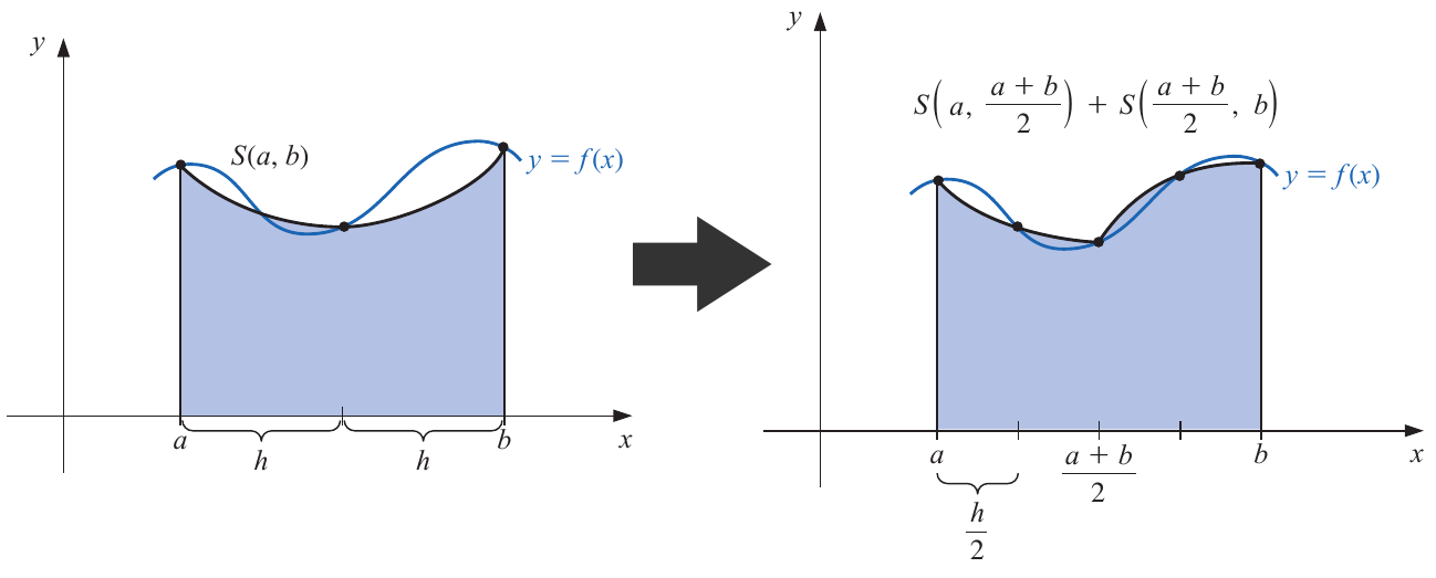
Now, instead of using an unique Simpson's quadrature, we implement two, by adding a new point in the midle of the interval $[a,b]$, $(a+b)/2$, yielding:

$$\int_a^bf(x)dx = S\left(a,\frac{a+b}{2}\right) + S\left(\frac{a+b}{2},b\right) - \frac{1}{16}\left(\frac{h^5}{90}\right)f^{(4)}(\xi)$$

For this expression, we reasonably assume an equal fourth-order derivative $f^{(4)}(\xi) = f^{(4)}(\xi_1) = f^{(4)}(\xi_2)$, where $\xi_1$ is the estimative for the first subtinterval (i.e. $\xi_1\in[a,(a+b)/2]$), and $\xi_2$ for the second one (i.e. $\xi_1\in[(a+b)/2, b]$).

As both expressions can approximate the real value of the integrate, we can equal them, obtaining:

$$\int_a^bf(x)dx \begin{cases} \sim S(a,b) - \frac{h^5}{90}f^{(4)}(\xi)\\ \approx S\left(a,\frac{a+b}{2}\right) + S\left(\frac{a+b}{2},b\right) - \frac{1}{16}\left(\frac{h^5}{90}\right)f^{(4)}(\xi)\\ \end{cases}$$

which leads us to a simple way to estimate the error without knowing the fourth-order derivative, i.e.

$$\frac{h^5}{90}f^{(4)}(\xi) = \frac{16}{15}\left| S(a,b) - S\left(a,\frac{a+b}{2}\right) - S\left(\frac{a+b}{2},b\right) \right|$$

If we fix a precision $\epsilon$, such that the obtained error for the second iteration is smaller

$$\frac{1}{16}\frac{h^5}{90}f^{(4)}(\xi) < \epsilon$$

it implies:

$$\left| S(a,b) - S\left(a,\frac{a+b}{2}\right) - S\left(\frac{a+b}{2},b\right) \right|< 15 \epsilon$$

and

$$\left| \int_a^bf(x) dx- S\left(a,\frac{a+b}{2}\right) - S\left(\frac{a+b}{2},b\right) \right|< \epsilon$$

The second iteration is then $15$ times more precise than the first one.

Steps Simpson's adaptive quadrature

1. Give the function $f(x)$ to be integrated, the inverval $[a,b]$ and set a desired precision $\epsilon$.

2. Compute the next Simpsons's quadratures:

$$S(a,b),\ S\left(a,\frac{a+b}{2}\right),\ S\left(\frac{a+b}{2},b\right)$$

3. If

$$\frac{1}{15}\left| S(a,b) - S\left(a,\frac{a+b}{2}\right) - S\left(\frac{a+b}{2},b\right) \right|<\epsilon$$

then the integration is ready and is given by:

$$\int_a^bf(x) dx \approx S\left(a,\frac{a+b}{2}\right) + S\left(\frac{a+b}{2},b\right)$$

within the given precision.

4. If the previous step is not fulfilled, repeat from step 2 using as new intervals $[a,(a+b)/2]$ and $[(a+b)/2,b]$ and a new precision $\epsilon_1 = \epsilon/2$. Repeating until step 3 is fulfilled for all the subintervals.