numerical-calculus.ipynb

Kernel: Python 3 (ipykernel)

Numerical Calculus

Throughout this section and the next ones, we shall cover the topic of numerical calculus. Calculus has been identified since ancient times as a powerful toolkit for analysing and handling geometrical problems. Since differential calculus was developed by Newton and Leibniz (in its actual notation), many different applications have been found, at the point that most of the current science is founded on it (e.g. differential and integral equations). Due to the ever increasing complexity of analytical expressions used in physics and astronomy, their usage becomes more and more impractical, and numerical approaches are more than necessary when one wants to go deeper. This issue has been identified since long ago and many numerical techniques have been developed. We shall cover only the most basic schemes, but also providing a basis for more formal approaches.

---

• Class activities with CoCalc

---

Bibliography

• https://github.com/restrepo/Calculus

• Thomas J. Sargent John Stachurski, Python Programming for Quantitative Economics GitHub

---

• Numerical Differentiation

  • Example 1

  • (n+1)-point formula

  • Endpoint formulas

  • Midpoint formulas

• Numerical Integration

---

%pylab inline
import numpy as np
import scipy.interpolate as interp

%pylab is deprecated, use %matplotlib inline and import the required libraries.
Populating the interactive namespace from numpy and matplotlib

Numerical Differentiation

According to the formal definition of differentiation, given a function $f(x)$ such that $f(x)\in C^1[a,b]$, the first order derivative is given by

$$\frac{d}{dx}f(x) = f'(x) = \lim_{h\rightarrow 0} \frac{f(x+h)-f(x)}{h}$$

However, when $f(x)$ exhibits a complex form or is a numerical function (only a discrete set of points are known), this expression becomes unfeasible. In spite of this, this formula gives us a very first rough way to calculate numerical derivatives by taking a finite interval $h$, i.e.

$$f'(x) \approx \frac{f(x+h)-f(x)}{h}$$

where the function must be known at least in $x_0$ and $x_1 = x_0+h$, and $h$ should be small enough.

Example 1

Evaluate the first derivative of the next function using the previous numerical scheme at the point $x_0=2.0$ and using $h=0.5,\ 0.1,\ 0.05,...$

$f(x) = \sqrt{1+\cos^2(x)}$

Compare with the real function and plot the tangent line using the found values of the slope.

from scipy import misc

It is used as:

misc.derivative(func, x0, dx=1.0, n=1, args=(), order=3)

Parameters
func : function → Input function.
x0 : float → The point at which n-th derivative is found.
dx : float, optional → Spacing.
n : int, optional → Order of the derivative. Default is 1.
args : tuple, optional → Arguments
order : int, optional → Number of points to use, must be odd.

def f(x):
    return np.sqrt( 1+np.cos(x)**2 )
x0 = 2

Activity: We now check for the impact of the change of the spacing dx. Try from dx=0.5 and then small values

eval('np.cos(np.pi)/np.sqrt(2)')

-0.7071067811865475

for i in range(5):
    dx=eval(input('dx='))
    print( misc.derivative(f,x0,dx=dx) )

{"name":"stdin","output_type":"stream","text":"dx= 1\n"}

0.13526274947015327

{"name":"stdin","output_type":"stream","text":"dx= 0.1\n"}

0.3462499420237386

{"name":"stdin","output_type":"stream","text":"dx= 0.01\n"}

0.3493266965195363

{"name":"stdin","output_type":"stream","text":"dx= 1e-3\n"}

0.34935758881293744

{"name":"stdin","output_type":"stream","text":"dx= 1e-6\n"}

0.3493579009417047

Compare with:

misc.derivative(f,x0,dx=1E-8)

0.34935789816614715

$$f'(x)=-\frac{\cos x\sin x }{\sqrt{1+\cos^2x}}$$

fp=lambda x:-np.cos(x)*np.sin(x)/f(x)
fp(2)

0.3493579008690488

m=misc.derivative(f,x0,dx=1E-6)

$$y_0=f(x_0)=m x_0+b$$$$b=f(x_0)-m x_0$$

b=f(x0)-m*x0

xmin = 1.6
xmax = 2.4
x = np.linspace( xmin, xmax, 100 )
plt.plot( x, f(x), color="black", label="function", linewidth=1 )
plt.plot( x, m*x+b,"r--", label=f"derivative at $x={x0}$")
plt.plot(x0,f(x0),'y*',markersize=10)
plt.grid()
plt.legend(fontsize=15)
plt.xlabel('$x$',size=15)
plt.ylabel(r'$f(x) = \sqrt{1+\cos^2(x)}$',size=15)

Text(0, 0.5, '$f(x) = \\sqrt{1+\\cos^2(x)}$')

---

Implementation of the derivate of the function inside a full range

We now generalize the derivative function to allow the evaluation of the derivate in a full range of values. It will be designed such that the evaluation in just one point can be still possible. In this way, the new function can be used as a full replacement of derivative function.

To implement this function we need three keys ingredients of python:

1. try and except python progamming sctructure

2. Function definition with generic mandatory and optional arguments

3. Conversion of a float function into a vectorized fuction

try and except python progamming sctructure

First we introduce the try and except python progamming sctructure, wich is used to bypass one python error. For example a zero dimension array has not a shape attribute, so that the following error, of type IndexError, is generated:

(1,)[1]

---------------------------------------------------------------------------
IndexError                                Traceback (most recent call last)
Input In [20], in <cell line: 1>()
----> 1 (1,)[1]
IndexError: tuple index out of range

np.array(3)

array(3)

nn=np.array(3).shape[0]
nn

---------------------------------------------------------------------------
IndexError                                Traceback (most recent call last)
Input In [33], in <cell line: 1>()
----> 1 nn=np.array(3).shape[0]
      2 nn
IndexError: tuple index out of range

To bypass that error we use the following code:

x=3
len(3)

---------------------------------------------------------------------------
TypeError                                 Traceback (most recent call last)
/tmp/ipykernel_57720/4138546388.py in <module>
      1 x=3
----> 2 len(3)

TypeError: object of type 'int' has no len()

np.array([]).shape

(0,)

x='3' #[2,3] #3 #[2,3], array([])
try: 
    nn=np.array(x).shape[0]
except IndexError:
    nn=-1

so that nn takes the values assigned in the except part:

nn

2

---

Activity: A float has the method is_integer() to check if the decimal part is zero. Creates a function is_integer(x) which works even in the case that the number is already an integer

x=2.
x.is_integer()

True

x=2
x.is_integer()

---------------------------------------------------------------------------
AttributeError                            Traceback (most recent call last)
Input In [50], in <cell line: 2>()
      1 x=2
----> 2 x.is_integer()
AttributeError: 'int' object has no attribute 'is_integer'

x=2.3
x.is_integer()

False

isinstance(2,int)

True

Objetos:

str,int,float,list,dict

isinstance(2,list)

False

eval('hola')

---------------------------------------------------------------------------
NameError                                 Traceback (most recent call last)
Input In [58], in <cell line: 1>()
----> 1 eval('hola')
File <string>:1, in <module>
NameError: name 'hola' is not defined

eval('hola mundo')

Traceback (most recent call last):
  File ~/anaconda3/lib/python3.9/site-packages/IPython/core/interactiveshell.py:3369 in run_code
    exec(code_obj, self.user_global_ns, self.user_ns)
  Input In [59] in <cell line: 1>
    eval('hola mundo')
  File <string>:1
    hola mundo
         ^
SyntaxError: unexpected EOF while parsing

def is_integer(x):
    '''
    Returns true if x is integer even if x is integer
    '''
    try:
        return x.is_integer()
    except AttributeError:
        if isinstance(x,int):
            return True
        elif isinstance(x,str):
            try:
                #recursive
                return is_integer(eval(x))
            except (NameError,SyntaxError):
                return False
        else:
            return False

## Test the functions for typical cases        
assert is_integer(3.)
assert is_integer(3.5)==False
assert is_integer(3)
assert is_integer('3')
assert is_integer('3+9+11')
assert is_integer('3.5')==False
assert is_integer('a')==False
assert is_integer('a b')==False
assert is_integer('1/2+1/2')
assert is_integer([1,3,5])==False
assert is_integer({'A':1})==False

Testing

assert True

assert False

---------------------------------------------------------------------------
AssertionError                            Traceback (most recent call last)
Input In [61], in <cell line: 1>()
----> 1 assert False
AssertionError: 

assert is_integer(3)

True

assert is trivial for True

assert generates an error for False

---

Function parameters

In python the function can be defined with mandatory and optional arguments

def f(a,b,c=2,d=3):
    return a+b-c+d

• a,b: is like a tuple of mandatory arguments → (a,b)

• c=2,d=3: is like a dictionary of optional arguments → {'c':2,'d':3}

Function definition with generic mandatory and optional arguments

We need to introduce another important concept about functions. There is a powerfull way to define a function with generic arguments:

1. Instead of the mandatory arguments we can use the generic list pointer: *args

2. Instead of the optional arguments we can use the generic dictionary pointer: **kwargs

def f(*args,**kwargs):
    if args:
        print('*args is the tuple of mandatory arguments: {}'.format(args))
        print('This allows to have a dynamic return according to input:')
        return type(args[0])
    if kwargs:
        print('*kwargs is the dictionary of optional arguments: {}'.format(kwargs))
        print('This allows to have a dynamic return according to input:')
        return type(list(kwargs.keys())[0]),type(list(kwargs.values())[0])

---

Activity; Check the function with any type of mandatory or optional argument

• Check the function without arguments

f()

• Check the function with a mandatory argument

f('hola mundo')

*args is the tuple of mandatory arguments: ('hola mundo',)
This allows to have a dynamic return according to input:

str

• Check the function with several mandatory arguments

f(2,[1,2],1+3j)

*args is the tuple of mandatory arguments: (2, [1, 2], (1+3j))
This allows to have a dynamic return according to input:

int

• Check the function with several optional arguments

• Check the function with one of the optional arguments equal to some list

f(d=3,h=[1,2],k='kk')

*kwargs is the dictionary of optional arguments: {'d': 3, 'h': [1, 2], 'k': 'kk'}
This allows to have a dynamic return according to input:

(str, int)

• Check the function with one string as mandatory argument, and with one of the optional arguments equal to some list

Conversion of a float function into a vectorized function

An important numpy function is:

Which convert a function which takes a float as an argument into a new function which que takes numpy arrays as an argument. The problem is that the converted function does not longer return a float when the argument is a float:

It is used as:

np.vectorize(pyfunc,...)

Parameters: pyfunc: A python function or method.

...

import math as m
m.sin(0.5)

0.479425538604203

m.sin([0.5,0.7])

---------------------------------------------------------------------------
TypeError                                 Traceback (most recent call last)
Input In [80], in <cell line: 1>()
----> 1 m.sin([0.5,0.7])
TypeError: must be real number, not list

import math as m
sin=np.vectorize(m.sin)
sin([0.5,0.7])

array([0.47942554, 0.64421769])

sin(0.5)

array(0.47942554)

Vectorization of Scipy method derivative

The problem is that derivative only works for one a point

misc.derivative(np.sin,1,dx=1E-6)

0.5403023058958567

misc.derivative(np.sin,[1,1.2],dx=1E-6)

---------------------------------------------------------------------------
TypeError                                 Traceback (most recent call last)
Input In [84], in <cell line: 1>()
----> 1 misc.derivative(np.sin,[1,1.2],dx=1E-6)
File ~/anaconda3/lib/python3.9/site-packages/scipy/misc/_common.py:144, in derivative(func, x0, dx, n, args, order)
    142 ho = order >> 1
    143 for k in range(order):
--> 144     val += weights[k]*func(x0+(k-ho)*dx,*args)
    145 return val / prod((dx,)*n,axis=0)
TypeError: can only concatenate list (not "float") to list

This is easily fixed with np.vectorize

derivative=np.vectorize(misc.derivative)

derivative(np.sin,[1,1.2],dx=1E-6)

array([0.54030231, 0.36235775])

derivative(np.sin,1,dx=1E-6)

array(0.54030231)

misc.derivative(np.sin,1,dx=1E-6)

0.5403023058958567

Code for the derivate of the function inside a full range

To recover the evaluation of a float into a float we can force the IndexError in order to use of the pure scipy derivative function when a float is given as input. The full implemention combine the three previos ingredients into a very compact pythonic-way function definition as shwon below

%pylab inline

import numpy as np
from scipy import misc
def derivative(func,x0,**kwargs):
    '''
    Vectorized replacement of scipy.misc derivative:
        from scipy.misc import derivative
    For usage check the derivative help, e.g, in jupyter: 
        from scipy.misc import derivative
        derivative?
    '''
    try:
        #x0: can be an array or a list  
        nn=np.asarray(x0).shape[0] ## force error if float is used 
        fp=np.vectorize(misc.derivative)
    except IndexError:
        fp=misc.derivative
        
    return fp(func,x0,**kwargs)

assert isinstance(derivative(np.sin,1,dx=1E-6),float)

import numpy as np
A=np.array([2])
type(A[0])

numpy.int64

numbers.Real

numbers.Real

import numbers
x=2#A[0]
isinstance(x, numbers.Real)#numbers.Integral)

True

import numpy as np
from scipy import misc
def derivative(func,x0,**kwargs):
    '''
    Vectorized replacement of scipy.misc derivative:
        from scipy.misc import derivative
    For usage check the derivative help, e.g, in jupyter: 
        from scipy.misc import derivative
        derivative?
    '''
    try:
        #x0: can be an array or a list  
        nn=np.asarray(x0).shape[0] ## force error if float is used 
        fp=np.vectorize(misc.derivative)
    except IndexError:
        fp=misc.derivative
        
    return fp(func,x0,**kwargs)

assert isinstance(derivative(np.sin,1,dx=1E-6),float)

which behaves exactly as the scipy derivative function when a float argument is used:

derivative(np.sin,1,dx=1E-6)

0.5403023058958567

derivative(np.sin,[1,1.5],dx=1E-6)

array([0.54030231, 0.0707372 ])

and as a vectorized function when an array argument is used:

misc.derivative(np.sin,1,dx=1E-6),misc.derivative(np.sin,1.5,dx=1E-6)

(0.5403023058958567, 0.0707372017072494)

derivative(np.sin,[1.,1.5],dx=1E-6)

array([0.54030231, 0.0707372 ])

derivative(np.sin,[1.,1.5],dx=1E-6,n=4,order=5)

array([-7.77156117e+08, -1.11022302e+09])

Let see now the implementation of the derivate function as full replacement of the derivative function:

Test

Let us check the implementation with the previous function

func=lambda x: np.sqrt( 1+np.cos(x)**2 )

but now evaluated for a list of values

x=[1.8,2,2.2]
funcp=derivative(func,x,dx=1E-3)
funcp

array([0.21576117, 0.34935759, 0.41006125])

For the prevous X array:

x0 = 2
xmin = 1.6
xmax = 2.4

x = np.linspace( xmin, xmax, 100 )

We have:

derivative(func,x,dx=1E-3).shape

(100,)

xmin = 1.6
xmax = 2.4

X = np.linspace( xmin, xmax, 100 )

plt.plot( X, func(X) , color="black", label="$f(x)$", linewidth=3)
plt.plot( X, derivative(func,X,dx=1E-3), color="red", label="$f'(x)$", linewidth=3)
plt.plot( X, derivative(func,X,dx=1E-3,n=2), color="blue", label="$f''(x)$", linewidth=3)
plt.legend(loc='best',fontsize=15)
plt.xlabel('$x$',size=15)
plt.grid()

Example

Finally we check the function $f(x)=\cos x$ in the range $[0,2\pi]$

xmin = 0
xmax = 2*np.pi

X = np.linspace( xmin, xmax, 100 )

plt.plot( X, np.cos(X) , "g-", label="$f(x)=\cos x$", linewidth=3)
plt.plot( X, derivative(np.cos,X,dx=1E-3), color="red", label="$f'(x)$", linewidth=3)
plt.plot( X, -np.sin(X) , 'b:', label="$-\sin x$", linewidth=3, zorder=10 )
plt.plot( X, derivative(np.cos,X,dx=1E-3,n=4,order=5), 'k:', label="$f^{(iv)}(x)$", linewidth=3)
plt.legend(loc='best',fontsize=15)
plt.xlabel('$x$',size=15)

Text(0.5, 0, '$x$')

misc.derivative(np.cos,np.pi/2,n=4,dx=1E-3,order=5)

-1.3010426069826051e-06

Activity: Implement the full derivative function by using isinstance() instead of try and except

from scipy import misc

def derivate(func,x0,**kwargs):
    '''
    Vectorized replacement of scipy.misc derivative:
        from scipy.misc import derivative
    For usage check the derivative help, e.g, in jupyter: 
        from scipy.misc import derivative
        derivative?
    '''
    if isinstance(x0,list): ## or ... or ...
        print(x0)
        fp=np.vectorize(misc.derivative)
    else:
        fp=misc.derivative
    return fp(func,x0,**kwargs)

isinstance( np.array([2,3]),numpy.ndarray )

True

derivate(np.cos,np.array([2,3]),dx=1E-6)

array([-0.90929743, -0.14112001])

Example: Heat transfer in a 1D bar

Fourier's Law of thermal conduction describes the diffusion of heat. Situations in which there are gradients of heat, a flux that tends to homogenise the temperature arises as a consequence of collisions of particles within a body. The Fourier's Law is giving by

$$q = -k\nabla T = -k\left( \frac{dT}{dx}\hat{i} + \frac{dT}{dy}\hat{j} + \frac{dT}{dz}\hat{k}\right)$$

where T is the temperature, $\nabla T$ its gradient and k is the material's conductivity. In the next example it is shown the magnitud of the heat flux in a 1D bar(wire).

def Temp(x):
    return x**3 + 3*x-1

Xn = np.linspace(0,10,100)

#Temperature profile 
def Temp(x):
    return x**3 + 3*x-1

## Points where function is known
Xn = np.linspace(0,10,100)

plt.figure( figsize=(8,7) )
plt.plot(Xn,derivate(Temp,Xn)*10)

plt.grid()
plt.xlabel( "$x$",fontsize =15 )
plt.ylabel( r"$\frac{dT}{dx}$",fontsize =20 )
plt.title( " Magnitud heat flux transfer in 1D bar" )

Text(0.5,1,' Magnitud heat flux transfer in 1D bar')

Activity

Construct a density map of the magnitud of the heat flux of a 2D bar. Consider the temperature profile as $$T(x,y) = x^3 + 3x-1+y^2$$

Activity

The Poisson's equation relates the matter content of a body with the gravitational potential through the next equation

$$\nabla^2 \phi = 4\pi G \rho$$$$\frac{1}{r^2}\frac{d}{dr}\left(r^2\frac{d\phi}{dr}\right)= 4\pi G \rho$$

where $\phi$ is the potential, $\rho$ the density and $G$ the gravitational constant.

Taking these data and using the three-point Midpoint formula, find the density field from the potential (seventh column in the file) and plot it against the radial coordinate. (Tip: Use $G=1$)

Activity

The radar stations A and B, separated by the distance a = 500 m, track the plane C by recording the angles $\alpha$ and $\beta$ at 1-second intervals. The successive readings are

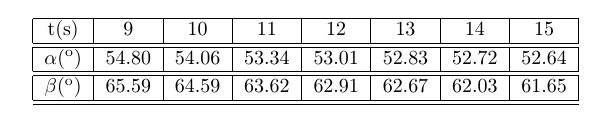
calculate the speed v using the 3 point approximantion at t = 10 ,12 and 14 s. Calculate the x component of the acceleration of the plane at = 12 s. The coordinates of the plane can be shown to be

$$\begin{equation} x = a\frac{\tan \beta}{\tan \beta- \tan \alpha}\\ y = a\frac{\tan \alpha\tan \beta}{\tan \beta- \tan \alpha} \end{equation}$$

---

Numerical Integration

Appendix

One implementation of derivative algorithm

#Function to evaluate
def function(x):
    return np.sqrt( 1+np.cos(x)**2 )

#X value
x0 = 2
xmin = 1.8
xmax = 2.2
#h step
hs = [0.5,0.1,0.05]

#Calculating derivatives
dfs = []
for h in hs:
    dfs.append( (function(x0+h)-function(x0))/h )
    
#Plotting
plt.figure( figsize=(10,8) )
#X array
X = np.linspace( xmin, xmax, 100 )
Y = function(X)
plt.plot( X, Y, color="black", label="function", linewidth=3, zorder=10 )
#Slopes
Xslp = [1,x0,3]
Yslp = [0,0,0]
for df, h in zip(dfs, hs):
    #First point
    Yslp[0] = function(x0)+df*(Xslp[0]-Xslp[1])
    #Second point
    Yslp[1] = function(x0)
    #Third point
    Yslp[2] = function(x0)+df*(Xslp[2]-Xslp[1])
    #Plotting this slope
    plt.plot( Xslp, Yslp, linewidth = 2, label="slope$=%1.2f$ for $h=%1.2f$"%(df,h) )

#Format
plt.grid()
plt.xlabel("x")
plt.ylabel("y")
plt.xlim( xmin, xmax )
plt.ylim( 1, 1.15 )
plt.legend( loc = "upper left" )

<matplotlib.legend.Legend at 0x7f2790fe7990>

n+1-point formula

A generalization of the previous formula is given by the (n+1)-point formula, where first-order derivatives are calculated using more than one point, what makes it a much better approximation for many problems. it is controled by the order option of the derivative function of scipy.misc

Theorem

For a function $f(x)$ such that $f(x)\in C^{n+1}[a,b]$, the next expression is always satisfied

$$f(x) = P(x) + \frac{f^{(n+1)}(\xi(x))}{(n+1)!}(x-x_0)(x-x_1)\cdots(x-x_n)$$

where $\{x_i\}_i$ is a set of point where the function is mapped, $\xi(x)$ is some function of $x$ such that $\xi\in[a,b]$, and $P(x)$ is the associated Lagrange interpolant polynomial.

As $n$ becomes higher, the approximation should be better as the error term becomes neglectable.

Taking the previous expression, and differenciating, we obtain

$$f(x) = \sum_{k=0}^n f(x_k)L_{n,k}(x) + \frac{(x-x_0)(x-x_1)\cdots(x-x_n)}{(n+1)!}f^{(n+1)}(\xi(x))$$$$f'(x_j) = \sum_{k=0}^n f(x_k)L'_{n,k}(x_j) + \frac{f^{(n+1)}(\xi(x_j))}{(n+1)!} \prod_{k=0,k\neq j}^{n}(x_j-x_k)$$

where $L_{n,k}$ is the $k$-th Lagrange basis functions for $n$ points, $L'_{n,k}$ is its first derivative.

Note that the last expressions is evaluated in $x_j$ rather than a general $x$ value, the cause of this is because this expression is not longer valid for another value not within the set $\{x_i\}_i$, however this is not an inconvenient when handling real applications.

This formula constitutes the (n+1)-point approximation and it comprises a generalization of almost all the existing schemes to differentiate numerically. Next, we shall derive some very used formulas.

For example, the form that takes this derivative polynomial for 3 points $(x_i,y_i)$ is the following

$$f'(x_j) = f(x_0)\left[ \frac{2x_j-x_1-x_2}{(x_0-x_1)(x_0-x_2)}\right] + f(x_1)\left[ \frac{2x_j-x_0-x_2}{(x_1-x_0)(x_1-x_2)}\right] + f(x_2)\left[ \frac{2x_j-x_0-x_1}{(x_2-x_0)(x_2-x_1)}\right]$$$$\hspace{2cm} + \frac{1}{6} f^{(3)}(\epsilon_j) \prod_{k=0,k\neq j}^{n}(x_j-x_k)$$

Endpoint formulas

Endpoint formulas are based on evaluating the derivative at the first of a set of points, i.e., if we want to evaluate $f'(x)$ at $x_i$, we then need $(x_i$, $x_{i+1}=x_i+h$, $x_{i+2}=x_i+2h$, $\cdots)$. For the sake of simplicity, it is usually assumed that the set $\{x_i\}_i$ is equally spaced such that $x_k = x_0+k\cdot h$.

Three-point Endpoint Formula

$$f'(x_i) = \frac{1}{2h}[-3f(x_i)+4f(x_i+h)-f(x_i+2h)] + \frac{h^2}{3}f^{(3)}(\xi)$$

with $\xi\in[x_i,x_i+2h]$

Five-point Endpoint Formula

$$f'(x_i) = \frac{1}{12h}[-25f(x_i)+48f(x_i+h)-36f(x_i+2h)+16f(x_i+3h)-3f(x_i+4h)] + \frac{h^4}{5}f^{(5)}(\xi)$$

with $\xi\in[x_i,x_i+4h]$

Endpoint formulas are especially useful near to the end of a set of points, where no further points exist.

Midpoint formulas

On the other hand, Midpoint formulas are based on evaluating the derivative at the middle of a set of points, i.e., if we want to evaluate $f'(x)$ at $x_i$, we then need $(\cdots$, $x_{i-2} = x_i - 2h$, $x_{i-1} = x_i - h$, $x_i$, $x_{i+1}=x_i+h$, $x_{i+2}=x_i+2h$, $\cdots)$.

Three-point Midpoint Formula

$$f'(x_i) = \frac{1}{2h}[f(x_i+h)-f(x_i-h)] + \frac{h^2}{6}f^{(3)}(\xi)$$

with $\xi\in[x_i-h,x_i+h]$

Five-point Midpoint Formula

$$f'(x_i) = \frac{1}{12h}[f(x_i-2h)-8f(x_i-h)+8f(x_i+h)-f(x_i+2h)] + \frac{h^4}{30}f^{(5)}(\xi)$$

with $\xi\in[x_i-2h,x_i+2h]$

As Midpoint formulas required one iteration less than Endpoint ones, they are more often used for numerical applications. Furthermore, the round-off error is smaller as well. However, near to the end of a set of points, they are no longer useful as no further points exists, and Endpoint formulas are preferable.

Example with custom implementation

#Temperature profile 
def Temp(x):
    return x**3 + 3*x-1

#Derivative three end point 

def TEP( Yn,i, h=0.01,right=0 ):
    suma = -3*Yn[i]+4*Yn[i+(-1)**right*1]-Yn[i+(-1)**right*2]
    return suma/(2*h*(-1)**right)

#Derivative mid point 
def TMP( Ynh,Ynmh, h = 0.01 ):    
    return (Ynh-Ynmh)/(2*h)

## Points where function is known
Xn = np.linspace(0,10,100)
Tn = Temp(Xn)
#Magnitude of heat flux array
Q = np.zeros(len(Xn))
#Left end derivative
Q[0] = TEP(Tn,0)

#Mid point derivatives
index = len(Xn)-1
for i in xrange( 1,index ):    
    Q[i] =  TMP( Tn[i+1],Tn[i-1] )

#Right end derivative      
Q[-1] = TEP( Tn,index,right=1 ) 

#Plotting 
plt.figure( figsize=(8,7) )
plt.plot(Xn,Q)

plt.grid()
plt.xlabel( "x",fontsize =15 )
plt.ylabel( "$\\frac{dT}{dx}$",fontsize =20 )
plt.title( " Magnitud heat flux transfer in 1D bar" )

<matplotlib.text.Text at 0x7f87263de3d0>