pix2pix.ipynb

Kernel: Python 3

Copyright 2019 The TensorFlow Authors.

Licensed under the Apache License, Version 2.0 (the "License");

#@title Licensed under the Apache License, Version 2.0 (the "License");
# you may not use this file except in compliance with the License.
# You may obtain a copy of the License at
#
# https://www.apache.org/licenses/LICENSE-2.0
#
# Unless required by applicable law or agreed to in writing, software
# distributed under the License is distributed on an "AS IS" BASIS,
# WITHOUT WARRANTIES OR CONDITIONS OF ANY KIND, either express or implied.
# See the License for the specific language governing permissions and
# limitations under the License.

pix2pix: Image-to-image translation with a conditional GAN

View on TensorFlow.org

Run in Google Colab

View source on GitHub

Download notebook

This tutorial demonstrates how to build and train a conditional generative adversarial network (cGAN) called pix2pix that learns a mapping from input images to output images, as described in Image-to-image translation with conditional adversarial networks{:.external} by Isola et al. (2017). pix2pix is not application specific—it can be applied to a wide range of tasks, including synthesizing photos from label maps, generating colorized photos from black and white images, turning Google Maps photos into aerial images, and even transforming sketches into photos.

In this example, your network will generate images of building facades using the CMP Facade Database provided by the Center for Machine Perception{:.external} at the Czech Technical University in Prague{:.external}. To keep it short, you will use a preprocessed copy{:.external} of this dataset created by the pix2pix authors.

In the pix2pix cGAN, you condition on input images and generate corresponding output images. cGANs were first proposed in Conditional Generative Adversarial Nets (Mirza and Osindero, 2014)

The architecture of your network will contain:

• A generator with a U-Net{:.external}-based architecture.

• A discriminator represented by a convolutional PatchGAN classifier (proposed in the pix2pix paper{:.external}).

Note that each epoch can take around 15 seconds on a single V100 GPU.

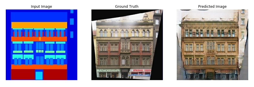
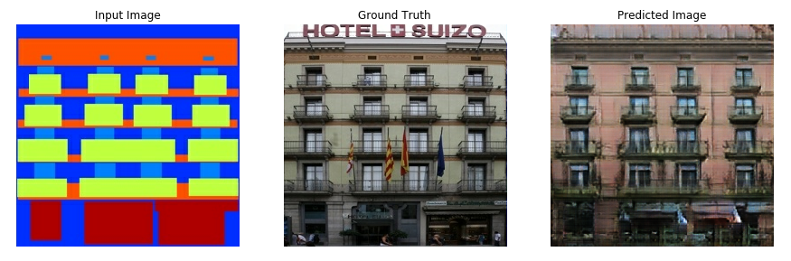
Below are some examples of the output generated by the pix2pix cGAN after training for 200 epochs on the facades dataset (80k steps).

Import TensorFlow and other libraries

import tensorflow as tf

import os
import pathlib
import time
import datetime

from matplotlib import pyplot as plt
from IPython import display

Load the dataset

Download the CMP Facade Database data (30MB). Additional datasets are available in the same format here{:.external}. In Colab you can select other datasets from the drop-down menu. Note that some of the other datasets are significantly larger (edges2handbags is 8GB in size).

dataset_name = "facades" #@param ["cityscapes", "edges2handbags", "edges2shoes", "facades", "maps", "night2day"]

_URL = f'http://efrosgans.eecs.berkeley.edu/pix2pix/datasets/{dataset_name}.tar.gz'

path_to_zip = tf.keras.utils.get_file(
    fname=f"{dataset_name}.tar.gz",
    origin=_URL,
    extract=True)

path_to_zip  = pathlib.Path(path_to_zip)

PATH = path_to_zip.parent/dataset_name

list(PATH.parent.iterdir())

Each original image is of size 256 x 512 containing two 256 x 256 images:

sample_image = tf.io.read_file(str(PATH / 'train/1.jpg'))
sample_image = tf.io.decode_jpeg(sample_image)
print(sample_image.shape)

plt.figure()
plt.imshow(sample_image)

You need to separate real building facade images from the architecture label images—all of which will be of size 256 x 256.

Define a function that loads image files and outputs two image tensors:

def load(image_file):
  # Read and decode an image file to a uint8 tensor
  image = tf.io.read_file(image_file)
  image = tf.io.decode_jpeg(image)

  # Split each image tensor into two tensors:
  # - one with a real building facade image
  # - one with an architecture label image 
  w = tf.shape(image)[1]
  w = w // 2
  input_image = image[:, w:, :]
  real_image = image[:, :w, :]

  # Convert both images to float32 tensors
  input_image = tf.cast(input_image, tf.float32)
  real_image = tf.cast(real_image, tf.float32)

  return input_image, real_image

Plot a sample of the input (architecture label image) and real (building facade photo) images:

inp, re = load(str(PATH / 'train/100.jpg'))
# Casting to int for matplotlib to display the images
plt.figure()
plt.imshow(inp / 255.0)
plt.figure()
plt.imshow(re / 255.0)

As described in the pix2pix paper{:.external}, you need to apply random jittering and mirroring to preprocess the training set.

Define several functions that:

1. Resize each 256 x 256 image to a larger height and width—286 x 286.

2. Randomly crop it back to 256 x 256.

3. Randomly flip the image horizontally i.e. left to right (random mirroring).

4. Normalize the images to the [-1, 1] range.

# The facade training set consist of 400 images
BUFFER_SIZE = 400
# The batch size of 1 produced better results for the U-Net in the original pix2pix experiment
BATCH_SIZE = 1
# Each image is 256x256 in size
IMG_WIDTH = 256
IMG_HEIGHT = 256

def resize(input_image, real_image, height, width):
  input_image = tf.image.resize(input_image, [height, width],
                                method=tf.image.ResizeMethod.NEAREST_NEIGHBOR)
  real_image = tf.image.resize(real_image, [height, width],
                               method=tf.image.ResizeMethod.NEAREST_NEIGHBOR)

  return input_image, real_image

def random_crop(input_image, real_image):
  stacked_image = tf.stack([input_image, real_image], axis=0)
  cropped_image = tf.image.random_crop(
      stacked_image, size=[2, IMG_HEIGHT, IMG_WIDTH, 3])

  return cropped_image[0], cropped_image[1]

# Normalizing the images to [-1, 1]
def normalize(input_image, real_image):
  input_image = (input_image / 127.5) - 1
  real_image = (real_image / 127.5) - 1

  return input_image, real_image

@tf.function()
def random_jitter(input_image, real_image):
  # Resizing to 286x286
  input_image, real_image = resize(input_image, real_image, 286, 286)

  # Random cropping back to 256x256
  input_image, real_image = random_crop(input_image, real_image)

  if tf.random.uniform(()) > 0.5:
    # Random mirroring
    input_image = tf.image.flip_left_right(input_image)
    real_image = tf.image.flip_left_right(real_image)

  return input_image, real_image

You can inspect some of the preprocessed output:

plt.figure(figsize=(6, 6))
for i in range(4):
  rj_inp, rj_re = random_jitter(inp, re)
  plt.subplot(2, 2, i + 1)
  plt.imshow(rj_inp / 255.0)
  plt.axis('off')
plt.show()

Having checked that the loading and preprocessing works, let's define a couple of helper functions that load and preprocess the training and test sets:

def load_image_train(image_file):
  input_image, real_image = load(image_file)
  input_image, real_image = random_jitter(input_image, real_image)
  input_image, real_image = normalize(input_image, real_image)

  return input_image, real_image

def load_image_test(image_file):
  input_image, real_image = load(image_file)
  input_image, real_image = resize(input_image, real_image,
                                   IMG_HEIGHT, IMG_WIDTH)
  input_image, real_image = normalize(input_image, real_image)

  return input_image, real_image

Build an input pipeline with tf.data

train_dataset = tf.data.Dataset.list_files(str(PATH / 'train/*.jpg'))
train_dataset = train_dataset.map(load_image_train,
                                  num_parallel_calls=tf.data.AUTOTUNE)
train_dataset = train_dataset.shuffle(BUFFER_SIZE)
train_dataset = train_dataset.batch(BATCH_SIZE)

try:
  test_dataset = tf.data.Dataset.list_files(str(PATH / 'test/*.jpg'))
except tf.errors.InvalidArgumentError:
  test_dataset = tf.data.Dataset.list_files(str(PATH / 'val/*.jpg'))
test_dataset = test_dataset.map(load_image_test)
test_dataset = test_dataset.batch(BATCH_SIZE)

Build the generator

The generator of your pix2pix cGAN is a modified U-Net{:.external}. A U-Net consists of an encoder (downsampler) and decoder (upsampler). (You can find out more about it in the Image segmentation tutorial and on the U-Net project website{:.external}.)

• Each block in the encoder is: Convolution -> Batch normalization -> Leaky ReLU

• Each block in the decoder is: Transposed convolution -> Batch normalization -> Dropout (applied to the first 3 blocks) -> ReLU

• There are skip connections between the encoder and decoder (as in the U-Net).

Define the downsampler (encoder):

OUTPUT_CHANNELS = 3

def downsample(filters, size, apply_batchnorm=True):
  initializer = tf.random_normal_initializer(0., 0.02)

  result = tf.keras.Sequential()
  result.add(
      tf.keras.layers.Conv2D(filters, size, strides=2, padding='same',
                             kernel_initializer=initializer, use_bias=False))

  if apply_batchnorm:
    result.add(tf.keras.layers.BatchNormalization())

  result.add(tf.keras.layers.LeakyReLU())

  return result

down_model = downsample(3, 4)
down_result = down_model(tf.expand_dims(inp, 0))
print (down_result.shape)

Define the upsampler (decoder):

def upsample(filters, size, apply_dropout=False):
  initializer = tf.random_normal_initializer(0., 0.02)

  result = tf.keras.Sequential()
  result.add(
    tf.keras.layers.Conv2DTranspose(filters, size, strides=2,
                                    padding='same',
                                    kernel_initializer=initializer,
                                    use_bias=False))

  result.add(tf.keras.layers.BatchNormalization())

  if apply_dropout:
      result.add(tf.keras.layers.Dropout(0.5))

  result.add(tf.keras.layers.ReLU())

  return result

up_model = upsample(3, 4)
up_result = up_model(down_result)
print (up_result.shape)

Define the generator with the downsampler and the upsampler:

def Generator():
  inputs = tf.keras.layers.Input(shape=[256, 256, 3])

  down_stack = [
    downsample(64, 4, apply_batchnorm=False),  # (batch_size, 128, 128, 64)
    downsample(128, 4),  # (batch_size, 64, 64, 128)
    downsample(256, 4),  # (batch_size, 32, 32, 256)
    downsample(512, 4),  # (batch_size, 16, 16, 512)
    downsample(512, 4),  # (batch_size, 8, 8, 512)
    downsample(512, 4),  # (batch_size, 4, 4, 512)
    downsample(512, 4),  # (batch_size, 2, 2, 512)
    downsample(512, 4),  # (batch_size, 1, 1, 512)
  ]

  up_stack = [
    upsample(512, 4, apply_dropout=True),  # (batch_size, 2, 2, 1024)
    upsample(512, 4, apply_dropout=True),  # (batch_size, 4, 4, 1024)
    upsample(512, 4, apply_dropout=True),  # (batch_size, 8, 8, 1024)
    upsample(512, 4),  # (batch_size, 16, 16, 1024)
    upsample(256, 4),  # (batch_size, 32, 32, 512)
    upsample(128, 4),  # (batch_size, 64, 64, 256)
    upsample(64, 4),  # (batch_size, 128, 128, 128)
  ]

  initializer = tf.random_normal_initializer(0., 0.02)
  last = tf.keras.layers.Conv2DTranspose(OUTPUT_CHANNELS, 4,
                                         strides=2,
                                         padding='same',
                                         kernel_initializer=initializer,
                                         activation='tanh')  # (batch_size, 256, 256, 3)

  x = inputs

  # Downsampling through the model
  skips = []
  for down in down_stack:
    x = down(x)
    skips.append(x)

  skips = reversed(skips[:-1])

  # Upsampling and establishing the skip connections
  for up, skip in zip(up_stack, skips):
    x = up(x)
    x = tf.keras.layers.Concatenate()([x, skip])

  x = last(x)

  return tf.keras.Model(inputs=inputs, outputs=x)

Visualize the generator model architecture:

generator = Generator()
tf.keras.utils.plot_model(generator, show_shapes=True, dpi=64)

Test the generator:

gen_output = generator(inp[tf.newaxis, ...], training=False)
plt.imshow(gen_output[0, ...])

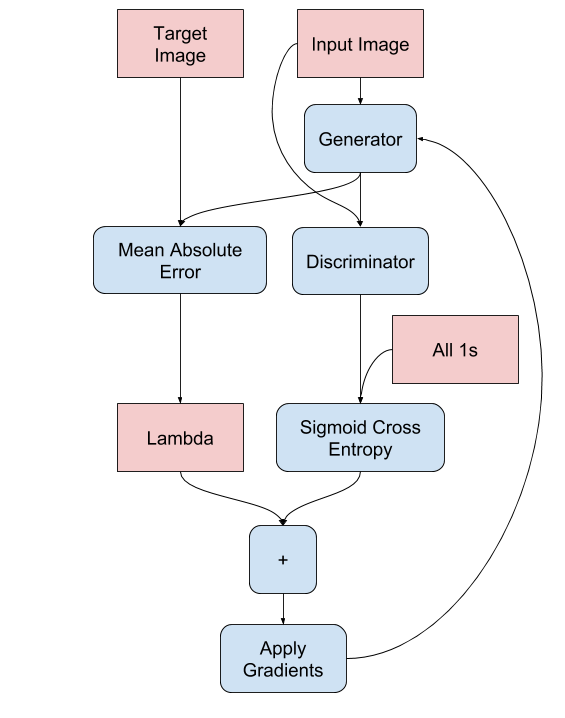
Define the generator loss

GANs learn a loss that adapts to the data, while cGANs learn a structured loss that penalizes a possible structure that differs from the network output and the target image, as described in the pix2pix paper{:.external}.

• The generator loss is a sigmoid cross-entropy loss of the generated images and an array of ones.

• The pix2pix paper also mentions the L1 loss, which is a MAE (mean absolute error) between the generated image and the target image.

• This allows the generated image to become structurally similar to the target image.

• The formula to calculate the total generator loss is gan_loss + LAMBDA * l1_loss, where LAMBDA = 100. This value was decided by the authors of the paper.

LAMBDA = 100

loss_object = tf.keras.losses.BinaryCrossentropy(from_logits=True)

def generator_loss(disc_generated_output, gen_output, target):
  gan_loss = loss_object(tf.ones_like(disc_generated_output), disc_generated_output)

  # Mean absolute error
  l1_loss = tf.reduce_mean(tf.abs(target - gen_output))

  total_gen_loss = gan_loss + (LAMBDA * l1_loss)

  return total_gen_loss, gan_loss, l1_loss

The training procedure for the generator is as follows:

Build the discriminator

The discriminator in the pix2pix cGAN is a convolutional PatchGAN classifier—it tries to classify if each image patch is real or not real, as described in the pix2pix paper{:.external}.

• Each block in the discriminator is: Convolution -> Batch normalization -> Leaky ReLU.

• The shape of the output after the last layer is (batch_size, 30, 30, 1).

• Each 30 x 30 image patch of the output classifies a 70 x 70 portion of the input image.

• The discriminator receives 2 inputs:

  • The input image and the target image, which it should classify as real.

  • The input image and the generated image (the output of the generator), which it should classify as fake.

  • Use tf.concat([inp, tar], axis=-1) to concatenate these 2 inputs together.

Let's define the discriminator:

def Discriminator():
  initializer = tf.random_normal_initializer(0., 0.02)

  inp = tf.keras.layers.Input(shape=[256, 256, 3], name='input_image')
  tar = tf.keras.layers.Input(shape=[256, 256, 3], name='target_image')

  x = tf.keras.layers.concatenate([inp, tar])  # (batch_size, 256, 256, channels*2)

  down1 = downsample(64, 4, False)(x)  # (batch_size, 128, 128, 64)
  down2 = downsample(128, 4)(down1)  # (batch_size, 64, 64, 128)
  down3 = downsample(256, 4)(down2)  # (batch_size, 32, 32, 256)

  zero_pad1 = tf.keras.layers.ZeroPadding2D()(down3)  # (batch_size, 34, 34, 256)
  conv = tf.keras.layers.Conv2D(512, 4, strides=1,
                                kernel_initializer=initializer,
                                use_bias=False)(zero_pad1)  # (batch_size, 31, 31, 512)

  batchnorm1 = tf.keras.layers.BatchNormalization()(conv)

  leaky_relu = tf.keras.layers.LeakyReLU()(batchnorm1)

  zero_pad2 = tf.keras.layers.ZeroPadding2D()(leaky_relu)  # (batch_size, 33, 33, 512)

  last = tf.keras.layers.Conv2D(1, 4, strides=1,
                                kernel_initializer=initializer)(zero_pad2)  # (batch_size, 30, 30, 1)

  return tf.keras.Model(inputs=[inp, tar], outputs=last)

Visualize the discriminator model architecture:

discriminator = Discriminator()
tf.keras.utils.plot_model(discriminator, show_shapes=True, dpi=64)

Test the discriminator:

disc_out = discriminator([inp[tf.newaxis, ...], gen_output], training=False)
plt.imshow(disc_out[0, ..., -1], vmin=-20, vmax=20, cmap='RdBu_r')
plt.colorbar()

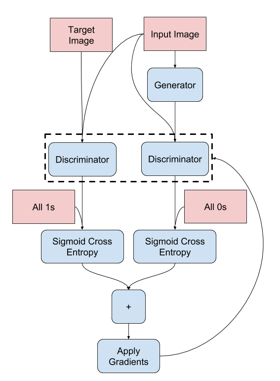
Define the discriminator loss

• The discriminator_loss function takes 2 inputs: real images and generated images.

• real_loss is a sigmoid cross-entropy loss of the real images and an array of ones(since these are the real images).

• generated_loss is a sigmoid cross-entropy loss of the generated images and an array of zeros (since these are the fake images).

• The total_loss is the sum of real_loss and generated_loss.

def discriminator_loss(disc_real_output, disc_generated_output):
  real_loss = loss_object(tf.ones_like(disc_real_output), disc_real_output)

  generated_loss = loss_object(tf.zeros_like(disc_generated_output), disc_generated_output)

  total_disc_loss = real_loss + generated_loss

  return total_disc_loss

The training procedure for the discriminator is shown below.

To learn more about the architecture and the hyperparameters you can refer to the pix2pix paper{:.external}.

Define the optimizers and a checkpoint-saver

generator_optimizer = tf.keras.optimizers.Adam(2e-4, beta_1=0.5)
discriminator_optimizer = tf.keras.optimizers.Adam(2e-4, beta_1=0.5)

checkpoint_dir = './training_checkpoints'
checkpoint_prefix = os.path.join(checkpoint_dir, "ckpt")
checkpoint = tf.train.Checkpoint(generator_optimizer=generator_optimizer,
                                 discriminator_optimizer=discriminator_optimizer,
                                 generator=generator,
                                 discriminator=discriminator)

Generate images

Write a function to plot some images during training.

• Pass images from the test set to the generator.

• The generator will then translate the input image into the output.

• The last step is to plot the predictions and voila!

Note: The training=True is intentional here since you want the batch statistics, while running the model on the test dataset. If you use training=False, you get the accumulated statistics learned from the training dataset (which you don't want).

def generate_images(model, test_input, tar):
  prediction = model(test_input, training=True)
  plt.figure(figsize=(15, 15))

  display_list = [test_input[0], tar[0], prediction[0]]
  title = ['Input Image', 'Ground Truth', 'Predicted Image']

  for i in range(3):
    plt.subplot(1, 3, i+1)
    plt.title(title[i])
    # Getting the pixel values in the [0, 1] range to plot.
    plt.imshow(display_list[i] * 0.5 + 0.5)
    plt.axis('off')
  plt.show()

Test the function:

for example_input, example_target in test_dataset.take(1):
  generate_images(generator, example_input, example_target)

Training

• For each example input generates an output.

• The discriminator receives the input_image and the generated image as the first input. The second input is the input_image and the target_image.

• Next, calculate the generator and the discriminator loss.

• Then, calculate the gradients of loss with respect to both the generator and the discriminator variables(inputs) and apply those to the optimizer.

• Finally, log the losses to TensorBoard.

log_dir="logs/"

summary_writer = tf.summary.create_file_writer(
  log_dir + "fit/" + datetime.datetime.now().strftime("%Y%m%d-%H%M%S"))

@tf.function
def train_step(input_image, target, step):
  with tf.GradientTape() as gen_tape, tf.GradientTape() as disc_tape:
    gen_output = generator(input_image, training=True)

    disc_real_output = discriminator([input_image, target], training=True)
    disc_generated_output = discriminator([input_image, gen_output], training=True)

    gen_total_loss, gen_gan_loss, gen_l1_loss = generator_loss(disc_generated_output, gen_output, target)
    disc_loss = discriminator_loss(disc_real_output, disc_generated_output)

  generator_gradients = gen_tape.gradient(gen_total_loss,
                                          generator.trainable_variables)
  discriminator_gradients = disc_tape.gradient(disc_loss,
                                               discriminator.trainable_variables)

  generator_optimizer.apply_gradients(zip(generator_gradients,
                                          generator.trainable_variables))
  discriminator_optimizer.apply_gradients(zip(discriminator_gradients,
                                              discriminator.trainable_variables))

  with summary_writer.as_default():
    tf.summary.scalar('gen_total_loss', gen_total_loss, step=step//1000)
    tf.summary.scalar('gen_gan_loss', gen_gan_loss, step=step//1000)
    tf.summary.scalar('gen_l1_loss', gen_l1_loss, step=step//1000)
    tf.summary.scalar('disc_loss', disc_loss, step=step//1000)

The actual training loop. Since this tutorial can run of more than one dataset, and the datasets vary greatly in size the training loop is setup to work in steps instead of epochs.

• Iterates over the number of steps.

• Every 10 steps print a dot (.).

• Every 1k steps: clear the display and run generate_images to show the progress.

• Every 5k steps: save a checkpoint.

def fit(train_ds, test_ds, steps):
  example_input, example_target = next(iter(test_ds.take(1)))
  start = time.time()

  for step, (input_image, target) in train_ds.repeat().take(steps).enumerate():
    if (step) % 1000 == 0:
      display.clear_output(wait=True)

      if step != 0:
        print(f'Time taken for 1000 steps: {time.time()-start:.2f} sec\n')

      start = time.time()

      generate_images(generator, example_input, example_target)
      print(f"Step: {step//1000}k")

    train_step(input_image, target, step)

    # Training step
    if (step+1) % 10 == 0:
      print('.', end='', flush=True)


    # Save (checkpoint) the model every 5k steps
    if (step + 1) % 5000 == 0:
      checkpoint.save(file_prefix=checkpoint_prefix)

This training loop saves logs that you can view in TensorBoard to monitor the training progress.

If you work on a local machine, you would launch a separate TensorBoard process. When working in a notebook, launch the viewer before starting the training to monitor with TensorBoard.

Launch the TensorBoard viewer (Sorry, this doesn't display on tensorflow.org):

%load_ext tensorboard
%tensorboard --logdir {log_dir}

You can view the results of a previous run of this notebook on TensorBoard.dev.

Finally, run the training loop:

fit(train_dataset, test_dataset, steps=40000)

Interpreting the logs is more subtle when training a GAN (or a cGAN like pix2pix) compared to a simple classification or regression model. Things to look for:

• Check that neither the generator nor the discriminator model has "won". If either the gen_gan_loss or the disc_loss gets very low, it's an indicator that this model is dominating the other, and you are not successfully training the combined model.

• The value log(2) = 0.69 is a good reference point for these losses, as it indicates a perplexity of 2 - the discriminator is, on average, equally uncertain about the two options.

• For the disc_loss, a value below 0.69 means the discriminator is doing better than random on the combined set of real and generated images.

• For the gen_gan_loss, a value below 0.69 means the generator is doing better than random at fooling the discriminator.

• As training progresses, the gen_l1_loss should go down.

Restore the latest checkpoint and test the network

!ls {checkpoint_dir}

# Restoring the latest checkpoint in checkpoint_dir
checkpoint.restore(tf.train.latest_checkpoint(checkpoint_dir))

Generate some images using the test set

# Run the trained model on a few examples from the test set
for inp, tar in test_dataset.take(5):
  generate_images(generator, inp, tar)