video_classification.ipynb

Kernel: Python 3

Copyright 2022 The TensorFlow Authors.

#@title Licensed under the Apache License, Version 2.0 (the "License");
# you may not use this file except in compliance with the License.
# You may obtain a copy of the License at
#
# https://www.apache.org/licenses/LICENSE-2.0
#
# Unless required by applicable law or agreed to in writing, software
# distributed under the License is distributed on an "AS IS" BASIS,
# WITHOUT WARRANTIES OR CONDITIONS OF ANY KIND, either express or implied.
# See the License for the specific language governing permissions and
# limitations under the License.

Ver en TensorFlow.org

Ejecutar en Google Colab

Ver fuente en GitHub

Descargar el bloc de notas

Clasificación de videos con una red neuronal convolucional 3D

Este tutorial demuestra el entrenamiento de una red neuronal convolucional 3D (CNN) para la clasificación de vídeos utilizando el conjunto de datos de reconocimiento de acciones UCF101. Una CNN 3D utiliza un filtro tridimensional para realizar las convoluciones. El núcleo puede deslizarse en tres direcciones, mientras que en una CNN 2D puede deslizarse en dos dimensiones. El modelo se basa en el trabajo publicado en A Closer Look at Spatiotemporal Convolutions for Action Recognition por D. Tran et al. (2017). En este tutorial, usted:

• Construirá una canalización de entrada

• Construirá un modelo de red neuronal convolucional 3D con conexiones residuales usando la API funcional de Keras

• Entrenará el modelo

• Evaluará y probará el modelo

Este video tutorial de clasificación es la segunda parte de una serie de video tutoriales de TensorFlow. Aquí están los otros tres tutoriales:

• Cargar datos de vídeo: Este tutorial explica gran parte del código usado en este documento.

• MoViNet para el reconocimiento de acciones en streaming: Familiarícese con los modelos MoViNet disponibles en TF Hub.

• Aprendizaje por transferencia para la clasificación de vídeo con MoViNet: Este tutorial explica cómo usar un modelo de clasificación de vídeo preentrenado y entrenado en un conjunto de datos diferente con el conjunto de datos UCF-101.

Preparación

Comience instalando e importando algunas librerías necesarias, incluyendo: remotezip para inspeccionar el contenido de un archivo ZIP, tqdm para usar una barra de progreso, OpenCV para procesar archivos de vídeo, einops para realizar operaciones tensoriales más complejas, y tensorflow_docs para incorporar datos en un bloc de notas de Jupyter.

Nota: Use TensorFlow 2.10 para ejecutar este tutorial. Es posible que las versiones superiores a TensorFlow 2.10 no se ejecuten correctamente.

!pip install remotezip tqdm opencv-python einops 
# Install TensorFlow 2.10
!pip install tensorflow==2.10.0

import tqdm
import random
import pathlib
import itertools
import collections

import cv2
import einops
import numpy as np
import remotezip as rz
import seaborn as sns
import matplotlib.pyplot as plt

import tensorflow as tf
import keras
from keras import layers

Carga y procesamiento de datos de video

La celda oculta inferior define funciones ayudantes para descargar una porción de datos del conjunto de datos UCF-101 y cargarla en un tf.data.Dataset. Puede aprender más sobre los pasos específicos del preprocesamiento en el tutorial Carga de datos de video, que le guiará a través de este código con más detalle.

La clase FrameGenerator al final del bloque oculto es la utilidad más importante en este caso. Crea un objeto iterable que puede alimentar los datos en la canalización de datos de TensorFlow. Específicamente, esta clase contiene un generador Python que carga los cuadros de video junto con su etiqueta codificada. La función del generador (__call__) produce el arreglo del marco emitido por frames_from_video_file y un vector codificado en un solo paso (one-hot) de la etiqueta asociada con el conjunto de cuadros.

#@title

def list_files_per_class(zip_url):
  """
    List the files in each class of the dataset given the zip URL.

    Args:
      zip_url: URL from which the files can be unzipped. 

    Return:
      files: List of files in each of the classes.
  """
  files = []
  with rz.RemoteZip(URL) as zip:
    for zip_info in zip.infolist():
      files.append(zip_info.filename)
  return files

def get_class(fname):
  """
    Retrieve the name of the class given a filename.

    Args:
      fname: Name of the file in the UCF101 dataset.

    Return:
      Class that the file belongs to.
  """
  return fname.split('_')[-3]

def get_files_per_class(files):
  """
    Retrieve the files that belong to each class. 

    Args:
      files: List of files in the dataset.

    Return:
      Dictionary of class names (key) and files (values).
  """
  files_for_class = collections.defaultdict(list)
  for fname in files:
    class_name = get_class(fname)
    files_for_class[class_name].append(fname)
  return files_for_class

def download_from_zip(zip_url, to_dir, file_names):
  """
    Download the contents of the zip file from the zip URL.

    Args:
      zip_url: Zip URL containing data.
      to_dir: Directory to download data to.
      file_names: Names of files to download.
  """
  with rz.RemoteZip(zip_url) as zip:
    for fn in tqdm.tqdm(file_names):
      class_name = get_class(fn)
      zip.extract(fn, str(to_dir / class_name))
      unzipped_file = to_dir / class_name / fn

      fn = pathlib.Path(fn).parts[-1]
      output_file = to_dir / class_name / fn
      unzipped_file.rename(output_file,)

def split_class_lists(files_for_class, count):
  """
    Returns the list of files belonging to a subset of data as well as the remainder of
    files that need to be downloaded.
    
    Args:
      files_for_class: Files belonging to a particular class of data.
      count: Number of files to download.

    Return:
      split_files: Files belonging to the subset of data.
      remainder: Dictionary of the remainder of files that need to be downloaded.
  """
  split_files = []
  remainder = {}
  for cls in files_for_class:
    split_files.extend(files_for_class[cls][:count])
    remainder[cls] = files_for_class[cls][count:]
  return split_files, remainder

def download_ufc_101_subset(zip_url, num_classes, splits, download_dir):
  """
    Download a subset of the UFC101 dataset and split them into various parts, such as
    training, validation, and test. 

    Args:
      zip_url: Zip URL containing data.
      num_classes: Number of labels.
      splits: Dictionary specifying the training, validation, test, etc. (key) division of data 
              (value is number of files per split).
      download_dir: Directory to download data to.

    Return:
      dir: Posix path of the resulting directories containing the splits of data.
  """
  files = list_files_per_class(zip_url)
  for f in files:
    tokens = f.split('/')
    if len(tokens) <= 2:
      files.remove(f) # Remove that item from the list if it does not have a filename
  
  files_for_class = get_files_per_class(files)

  classes = list(files_for_class.keys())[:num_classes]

  for cls in classes:
    new_files_for_class = files_for_class[cls]
    random.shuffle(new_files_for_class)
    files_for_class[cls] = new_files_for_class
    
  # Only use the number of classes you want in the dictionary
  files_for_class = {x: files_for_class[x] for x in list(files_for_class)[:num_classes]}

  dirs = {}
  for split_name, split_count in splits.items():
    print(split_name, ":")
    split_dir = download_dir / split_name
    split_files, files_for_class = split_class_lists(files_for_class, split_count)
    download_from_zip(zip_url, split_dir, split_files)
    dirs[split_name] = split_dir

  return dirs

def format_frames(frame, output_size):
  """
    Pad and resize an image from a video.
    
    Args:
      frame: Image that needs to resized and padded. 
      output_size: Pixel size of the output frame image.

    Return:
      Formatted frame with padding of specified output size.
  """
  frame = tf.image.convert_image_dtype(frame, tf.float32)
  frame = tf.image.resize_with_pad(frame, *output_size)
  return frame

def frames_from_video_file(video_path, n_frames, output_size = (224,224), frame_step = 15):
  """
    Creates frames from each video file present for each category.

    Args:
      video_path: File path to the video.
      n_frames: Number of frames to be created per video file.
      output_size: Pixel size of the output frame image.

    Return:
      An NumPy array of frames in the shape of (n_frames, height, width, channels).
  """
  # Read each video frame by frame
  result = []
  src = cv2.VideoCapture(str(video_path))  

  video_length = src.get(cv2.CAP_PROP_FRAME_COUNT)

  need_length = 1 + (n_frames - 1) * frame_step

  if need_length > video_length:
    start = 0
  else:
    max_start = video_length - need_length
    start = random.randint(0, max_start + 1)

  src.set(cv2.CAP_PROP_POS_FRAMES, start)
  # ret is a boolean indicating whether read was successful, frame is the image itself
  ret, frame = src.read()
  result.append(format_frames(frame, output_size))

  for _ in range(n_frames - 1):
    for _ in range(frame_step):
      ret, frame = src.read()
    if ret:
      frame = format_frames(frame, output_size)
      result.append(frame)
    else:
      result.append(np.zeros_like(result[0]))
  src.release()
  result = np.array(result)[..., [2, 1, 0]]

  return result

class FrameGenerator:
  def __init__(self, path, n_frames, training = False):
    """ Returns a set of frames with their associated label. 

      Args:
        path: Video file paths.
        n_frames: Number of frames. 
        training: Boolean to determine if training dataset is being created.
    """
    self.path = path
    self.n_frames = n_frames
    self.training = training
    self.class_names = sorted(set(p.name for p in self.path.iterdir() if p.is_dir()))
    self.class_ids_for_name = dict((name, idx) for idx, name in enumerate(self.class_names))

  def get_files_and_class_names(self):
    video_paths = list(self.path.glob('*/*.avi'))
    classes = [p.parent.name for p in video_paths] 
    return video_paths, classes

  def __call__(self):
    video_paths, classes = self.get_files_and_class_names()

    pairs = list(zip(video_paths, classes))

    if self.training:
      random.shuffle(pairs)

    for path, name in pairs:
      video_frames = frames_from_video_file(path, self.n_frames) 
      label = self.class_ids_for_name[name] # Encode labels
      yield video_frames, label

URL = 'https://storage.googleapis.com/thumos14_files/UCF101_videos.zip'
download_dir = pathlib.Path('./UCF101_subset/')
subset_paths = download_ufc_101_subset(URL, 
                        num_classes = 10, 
                        splits = {"train": 30, "val": 10, "test": 10},
                        download_dir = download_dir)

Cree los conjuntos de entrenamiento, validación y prueba (train_ds, val_ds y test_ds).

n_frames = 10
batch_size = 8

output_signature = (tf.TensorSpec(shape = (None, None, None, 3), dtype = tf.float32),
                    tf.TensorSpec(shape = (), dtype = tf.int16))

train_ds = tf.data.Dataset.from_generator(FrameGenerator(subset_paths['train'], n_frames, training=True),
                                          output_signature = output_signature)


# Batch the data
train_ds = train_ds.batch(batch_size)

val_ds = tf.data.Dataset.from_generator(FrameGenerator(subset_paths['val'], n_frames),
                                        output_signature = output_signature)
val_ds = val_ds.batch(batch_size)

test_ds = tf.data.Dataset.from_generator(FrameGenerator(subset_paths['test'], n_frames),
                                         output_signature = output_signature)

test_ds = test_ds.batch(batch_size)

Crear el modelo

El siguiente modelo de red neuronal convolucional 3D se basa en el artículo A Closer Look at Spatiotemporal Convolutions for Action Recognition de D. Tran et al. (2017). El artículo compara varias versiones de ResNets 3D. En lugar de operar sobre una sola imagen con dimensiones (height, width), como las ResNets estándares, estas operan sobre el volumen de vídeo (time, height, width). El enfoque más obvio a este problema sería reemplazar cada (layers.Conv2D) de convolución 2D por una convolución 3D (layers.Conv3D).

Este tutorial usa una convolución (2 + 1)D con conexiones residuales. La convolución (2 + 1)D permite descomponer las dimensiones espacial y temporal, creando así dos pasos separados. Una ventaja de este enfoque es que la factorización de las convoluciones en dimensiones espaciales y temporales ahorra parámetros.

Para cada ubicación de salida, una convolución 3D combina todos los vectores de un parche 3D del volumen para crear un vector en el volumen de salida.

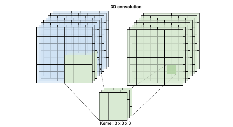
Esta operación toma entradas time * height * width * channels y produce salidas channels (suponiendo que el número de canales de entrada y de salida sea el mismo. Así, una capa de convolución 3D con un tamaño de kernel de (3 x 3 x 3) necesitaría una matriz de ponderación con entradas de 27 * canales ** 2. El documento de referencia encontró que un enfoque más eficaz y eficiente era factorizar la convolución. En lugar de una única convolución 3D para procesar las dimensiones temporal y espacial, propusieron una convolución "(2+1)D" que procesa las dimensiones espacial y temporal por separado. La figura siguiente muestra las convoluciones espacial y temporal factorizadas de una convolución (2 + 1)D.

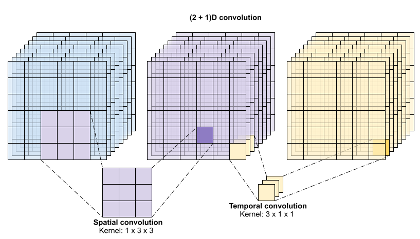
La principal ventaja de este enfoque es que reduce el número de parámetros. En la convolución (2 + 1)D, la convolución espacial toma datos de la forma (1, width, height), mientras que la convolución temporal toma datos de la forma (time, 1, 1). Por ejemplo, una convolución (2 + 1)D con tamaño de kernel (3 x 3 x 3) necesitaría matrices de ponderación de tamaño (9 * channels**2) + (3 * channels**2), menos de la mitad que la convolución 3D completa. Este tutorial implementa la ResNet18 (2 + 1)D, en la que cada convolución de la resnet se sustituye por una convolución (2+1)D.

# Define the dimensions of one frame in the set of frames created
HEIGHT = 224
WIDTH = 224

class Conv2Plus1D(keras.layers.Layer):
  def __init__(self, filters, kernel_size, padding):
    """
      A sequence of convolutional layers that first apply the convolution operation over the
      spatial dimensions, and then the temporal dimension. 
    """
    super().__init__()
    self.seq = keras.Sequential([  
        # Spatial decomposition
        layers.Conv3D(filters=filters,
                      kernel_size=(1, kernel_size[1], kernel_size[2]),
                      padding=padding),
        # Temporal decomposition
        layers.Conv3D(filters=filters, 
                      kernel_size=(kernel_size[0], 1, 1),
                      padding=padding)
        ])
  
  def call(self, x):
    return self.seq(x)

Un modelo ResNet se elabora a partir de una secuencia de bloques residuales. Un bloque residual tiene dos ramas. La rama principal realiza el cálculo, pero dificulta el paso de los gradientes. La derivación residual pasa por alto el cálculo principal y, en la mayoría de los casos, se limita a añadir la entrada a la salida de la rama principal. Los gradientes fluyen fácilmente a través de esta rama. Por lo tanto, habrá una ruta fácil desde la función de pérdida hasta cualquiera de las ramas principales del bloque residual. Esto evita el problema del gradiente evanescente.

Cree la rama principal del bloque residual con la siguiente clase. A diferencia de la estructura estándar de ResNet, ésta utiliza la capa personalizada Conv2Plus1D en lugar de layers.Conv2D.

class ResidualMain(keras.layers.Layer):
  """
    Residual block of the model with convolution, layer normalization, and the
    activation function, ReLU.
  """
  def __init__(self, filters, kernel_size):
    super().__init__()
    self.seq = keras.Sequential([
        Conv2Plus1D(filters=filters,
                    kernel_size=kernel_size,
                    padding='same'),
        layers.LayerNormalization(),
        layers.ReLU(),
        Conv2Plus1D(filters=filters, 
                    kernel_size=kernel_size,
                    padding='same'),
        layers.LayerNormalization()
    ])
    
  def call(self, x):
    return self.seq(x)

Para añadir la rama residual a la rama principal es necesario que tenga el mismo tamaño. La capa Project inferior se ocupa de los casos en los que se modifica el número de canales en la derivación. En concreto, se añade una secuencia de capa densamente conectada seguida de normalización.

class Project(keras.layers.Layer):
  """
    Project certain dimensions of the tensor as the data is passed through different 
    sized filters and downsampled. 
  """
  def __init__(self, units):
    super().__init__()
    self.seq = keras.Sequential([
        layers.Dense(units),
        layers.LayerNormalization()
    ])

  def call(self, x):
    return self.seq(x)

Use add_residual_block para crear una conexión de salto entre las capas del modelo.

def add_residual_block(input, filters, kernel_size):
  """
    Add residual blocks to the model. If the last dimensions of the input data
    and filter size does not match, project it such that last dimension matches.
  """
  out = ResidualMain(filters, 
                     kernel_size)(input)
  
  res = input
  # Using the Keras functional APIs, project the last dimension of the tensor to
  # match the new filter size
  if out.shape[-1] != input.shape[-1]:
    res = Project(out.shape[-1])(res)

  return layers.add([res, out])

Es necesario cambiar el tamaño del vídeo para realizar un downsampling de los datos. En concreto, el downsampling de los fotogramas de vídeo permite que el modelo examine partes concretas de los fotogramas para detectar patrones que puedan ser específicos de una determinada acción. Mediante el downsampling, se puede descartar la información no esencial. Además, redimensionar el vídeo permitirá reducir la dimensionalidad y, por tanto, acelerar el procesamiento a través del modelo.

class ResizeVideo(keras.layers.Layer):
  def __init__(self, height, width):
    super().__init__()
    self.height = height
    self.width = width
    self.resizing_layer = layers.Resizing(self.height, self.width)

  def call(self, video):
    """
      Use the einops library to resize the tensor.  
      
      Args:
        video: Tensor representation of the video, in the form of a set of frames.
      
      Return:
        A downsampled size of the video according to the new height and width it should be resized to.
    """
    # b stands for batch size, t stands for time, h stands for height, 
    # w stands for width, and c stands for the number of channels.
    old_shape = einops.parse_shape(video, 'b t h w c')
    images = einops.rearrange(video, 'b t h w c -> (b t) h w c')
    images = self.resizing_layer(images)
    videos = einops.rearrange(
        images, '(b t) h w c -> b t h w c',
        t = old_shape['t'])
    return videos

Usa la API funcional Keras para construir la red residual.

input_shape = (None, 10, HEIGHT, WIDTH, 3)
input = layers.Input(shape=(input_shape[1:]))
x = input

x = Conv2Plus1D(filters=16, kernel_size=(3, 7, 7), padding='same')(x)
x = layers.BatchNormalization()(x)
x = layers.ReLU()(x)
x = ResizeVideo(HEIGHT // 2, WIDTH // 2)(x)

# Block 1
x = add_residual_block(x, 16, (3, 3, 3))
x = ResizeVideo(HEIGHT // 4, WIDTH // 4)(x)

# Block 2
x = add_residual_block(x, 32, (3, 3, 3))
x = ResizeVideo(HEIGHT // 8, WIDTH // 8)(x)

# Block 3
x = add_residual_block(x, 64, (3, 3, 3))
x = ResizeVideo(HEIGHT // 16, WIDTH // 16)(x)

# Block 4
x = add_residual_block(x, 128, (3, 3, 3))

x = layers.GlobalAveragePooling3D()(x)
x = layers.Flatten()(x)
x = layers.Dense(10)(x)

model = keras.Model(input, x)

frames, label = next(iter(train_ds))
model.build(frames)

# Visualize the model
keras.utils.plot_model(model, expand_nested=True, dpi=60, show_shapes=True)

Entrenar el modelo

Para este tutorial, seleccione el optimizador tf.keras.optimizers.Adam y la función de pérdida tf.keras.losses.SparseCategoricalCrossentropy. Use el argumento metrics para ver la precisión del rendimiento del modelo en cada paso.

model.compile(loss = keras.losses.SparseCategoricalCrossentropy(from_logits=True), 
              optimizer = keras.optimizers.Adam(learning_rate = 0.0001), 
              metrics = ['accuracy'])

Entrene el modelo durante 50 épocas con el método Model.fit de Keras.

Nota: Este modelo de ejemplo se entrena con menos puntos de datos (300 ejemplos de entrenamiento y 100 de validación) para mantener un tiempo de entrenamiento razonable para este tutorial. Además, este modelo de ejemplo puede tardar más de una hora en entrenarse.

history = model.fit(x = train_ds,
                    epochs = 50, 
                    validation_data = val_ds)

Visualizar los resultados

Cree gráficos de la pérdida y la precisión en los conjuntos de entrenamiento y validación:

def plot_history(history):
  """
    Plotting training and validation learning curves.

    Args:
      history: model history with all the metric measures
  """
  fig, (ax1, ax2) = plt.subplots(2)

  fig.set_size_inches(18.5, 10.5)

  # Plot loss
  ax1.set_title('Loss')
  ax1.plot(history.history['loss'], label = 'train')
  ax1.plot(history.history['val_loss'], label = 'test')
  ax1.set_ylabel('Loss')
  
  # Determine upper bound of y-axis
  max_loss = max(history.history['loss'] + history.history['val_loss'])

  ax1.set_ylim([0, np.ceil(max_loss)])
  ax1.set_xlabel('Epoch')
  ax1.legend(['Train', 'Validation']) 

  # Plot accuracy
  ax2.set_title('Accuracy')
  ax2.plot(history.history['accuracy'],  label = 'train')
  ax2.plot(history.history['val_accuracy'], label = 'test')
  ax2.set_ylabel('Accuracy')
  ax2.set_ylim([0, 1])
  ax2.set_xlabel('Epoch')
  ax2.legend(['Train', 'Validation'])

  plt.show()

plot_history(history)

Evaluar el modelo

Usar Model.evaluate de Keras para conocer la pérdida y la precisión en el conjunto de datos de prueba.

Nota: El modelo de ejemplo de este tutorial usa un subgrupo del conjunto de datos UCF101 para mantener un tiempo de entrenamiento razonable. La precisión y la pérdida pueden mejorarse con un mayor ajuste de hiperparámetros o con más datos de entrenamiento.

model.evaluate(test_ds, return_dict=True)

Para visualizar mejor el rendimiento del modelo, use una matriz de confusión. La matriz de confusión le permite evaluar el rendimiento del modelo de clasificación más allá de la precisión. Para construir la matriz de confusión para este problema de clasificación multiclase, obtenga los valores reales en el conjunto de pruebas y los valores predichos.

def get_actual_predicted_labels(dataset): 
  """
    Create a list of actual ground truth values and the predictions from the model.

    Args:
      dataset: An iterable data structure, such as a TensorFlow Dataset, with features and labels.

    Return:
      Ground truth and predicted values for a particular dataset.
  """
  actual = [labels for _, labels in dataset.unbatch()]
  predicted = model.predict(dataset)

  actual = tf.stack(actual, axis=0)
  predicted = tf.concat(predicted, axis=0)
  predicted = tf.argmax(predicted, axis=1)

  return actual, predicted

def plot_confusion_matrix(actual, predicted, labels, ds_type):
  cm = tf.math.confusion_matrix(actual, predicted)
  ax = sns.heatmap(cm, annot=True, fmt='g')
  sns.set(rc={'figure.figsize':(12, 12)})
  sns.set(font_scale=1.4)
  ax.set_title('Confusion matrix of action recognition for ' + ds_type)
  ax.set_xlabel('Predicted Action')
  ax.set_ylabel('Actual Action')
  plt.xticks(rotation=90)
  plt.yticks(rotation=0)
  ax.xaxis.set_ticklabels(labels)
  ax.yaxis.set_ticklabels(labels)

fg = FrameGenerator(subset_paths['train'], n_frames, training=True)
labels = list(fg.class_ids_for_name.keys())

actual, predicted = get_actual_predicted_labels(train_ds)
plot_confusion_matrix(actual, predicted, labels, 'training')

actual, predicted = get_actual_predicted_labels(test_ds)
plot_confusion_matrix(actual, predicted, labels, 'test')

Los valores de precisión y memoria de cada clase también pueden calcularse utilizando una matriz de confusión.

def calculate_classification_metrics(y_actual, y_pred, labels):
  """
    Calculate the precision and recall of a classification model using the ground truth and
    predicted values. 

    Args:
      y_actual: Ground truth labels.
      y_pred: Predicted labels.
      labels: List of classification labels.

    Return:
      Precision and recall measures.
  """
  cm = tf.math.confusion_matrix(y_actual, y_pred)
  tp = np.diag(cm) # Diagonal represents true positives
  precision = dict()
  recall = dict()
  for i in range(len(labels)):
    col = cm[:, i]
    fp = np.sum(col) - tp[i] # Sum of column minus true positive is false negative
    
    row = cm[i, :]
    fn = np.sum(row) - tp[i] # Sum of row minus true positive, is false negative
    
    precision[labels[i]] = tp[i] / (tp[i] + fp) # Precision 
    
    recall[labels[i]] = tp[i] / (tp[i] + fn) # Recall
  
  return precision, recall

precision, recall = calculate_classification_metrics(actual, predicted, labels) # Test dataset

precision

recall

Siguientes pasos

Para más información sobre cómo trabajar con datos de video en TensorFlow, consulte los siguientes tutoriales:

• Carga de datos de video

• MoViNet para reconocimiento de acciones de transmisión

• Aprendizaje por transferencia para clasificación de video con MoViNet