GitHub Repository: tensorflow/docs-l10n
Path: blob/master/site/ja/addons/tutorials/losses_triplet.ipynb
²⁵¹¹⁸ views

Kernel: Python 3

Copyright 2020 The TensorFlow Authors.

In [ ]:

#@title Licensed under the Apache License, Version 2.0
# you may not use this file except in compliance with the License.
# You may obtain a copy of the License at
#
# https://www.apache.org/licenses/LICENSE-2.0
#
# Unless required by applicable law or agreed to in writing, software
# distributed under the License is distributed on an "AS IS" BASIS,
# WITHOUT WARRANTIES OR CONDITIONS OF ANY KIND, either express or implied.
# See the License for the specific language governing permissions and
# limitations under the License.

TensorFlow Addons 損失 : TripletSemiHardLoss

概要

このノートブックでは、TensorFlow Addons で TripletSemiHardLoss を使用する方法を紹介します。

リソース:

トリプレット損失

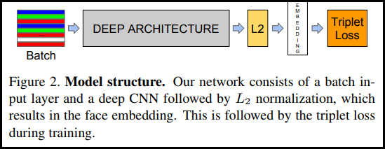
FaceNet の論文で初めて紹介されたトリプレット損失 (TripletLoss) は、異なるクラスの埋め込み間の距離を最大化しながら、同じクラスの特徴を密接に埋め込むようにニューラルネットワークをトレーニングする損失関数です。これを行うために、1 つのネガティブサンプルと 1 つのポジティブサンプルと共にアンカーが選択されます。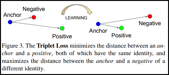 fig3

損失関数はユークリッド距離関数として記述されます。

Oliver Moindrot のブログでは、アルゴリズムがとてもよく詳説されています

ここで、A はアンカー入力、P はポジティブサンプル入力、N はネガティブサンプル入力、およびアルファは、トリプレットが「簡単」になり過ぎて重みを調整する必要がなくなった時に指定するマージンです。

セミハードオンライン学習

論文にあるように、最良の結果は「セミハード」として知られるトリプレットから得られます。これらはネガティブがポジティブよりアンカーから離れていても、ポジティブの損失を生成するトリプレットと定義されています。これらのトリプレットを効率的に見つけるために、オンライン学習を利用して、各バッチのセミハードの例のみからトレーニングします。

セットアップ

In [ ]:

!pip install -U tensorflow-addons

In [ ]:

import io
import numpy as np

In [ ]:

import tensorflow as tf
import tensorflow_addons as tfa
import tensorflow_datasets as tfds

データを準備する

In [ ]:

def _normalize_img(img, label):
    img = tf.cast(img, tf.float32) / 255.
    return (img, label)

train_dataset, test_dataset = tfds.load(name="mnist", split=['train', 'test'], as_supervised=True)

# Build your input pipelines
train_dataset = train_dataset.shuffle(1024).batch(32)
train_dataset = train_dataset.map(_normalize_img)

test_dataset = test_dataset.batch(32)
test_dataset = test_dataset.map(_normalize_img)

モデルを構築する

fig2

In [ ]:

model = tf.keras.Sequential([
    tf.keras.layers.Conv2D(filters=64, kernel_size=2, padding='same', activation='relu', input_shape=(28,28,1)),
    tf.keras.layers.MaxPooling2D(pool_size=2),
    tf.keras.layers.Dropout(0.3),
    tf.keras.layers.Conv2D(filters=32, kernel_size=2, padding='same', activation='relu'),
    tf.keras.layers.MaxPooling2D(pool_size=2),
    tf.keras.layers.Dropout(0.3),
    tf.keras.layers.Flatten(),
    tf.keras.layers.Dense(256, activation=None), # No activation on final dense layer
    tf.keras.layers.Lambda(lambda x: tf.math.l2_normalize(x, axis=1)) # L2 normalize embeddings

])

トレーニングして評価する

In [ ]:

# Compile the model
model.compile(
    optimizer=tf.keras.optimizers.Adam(0.001),
    loss=tfa.losses.TripletSemiHardLoss())

In [ ]:

# Train the network
history = model.fit(
    train_dataset,
    epochs=5)

In [ ]:

# Evaluate the network
results = model.predict(test_dataset)

In [ ]:

# Save test embeddings for visualization in projector
np.savetxt("vecs.tsv", results, delimiter='\t')

out_m = io.open('meta.tsv', 'w', encoding='utf-8')
for img, labels in tfds.as_numpy(test_dataset):
    [out_m.write(str(x) + "\n") for x in labels]
out_m.close()


try:
  from google.colab import files
  files.download('vecs.tsv')
  files.download('meta.tsv')
except:
  pass

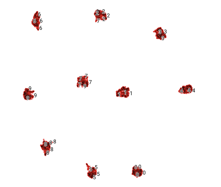
プロジェクターを埋め込む

ベクトルファイルとメタデータファイルは、次のリンクから読み込んで可視化することができます。https://projector.tensorflow.org/

埋め込んだテストデータを UMAP で可視化すると、その結果を見ることができます。 embedding