image_captioning.ipynb

Kernel: Python 3

Copyright 2018 The TensorFlow Authors.

#@title Licensed under the Apache License, Version 2.0 (the "License");
# you may not use this file except in compliance with the License.
# You may obtain a copy of the License at
#
# https://www.apache.org/licenses/LICENSE-2.0
#
# Unless required by applicable law or agreed to in writing, software
# distributed under the License is distributed on an "AS IS" BASIS,
# WITHOUT WARRANTIES OR CONDITIONS OF ANY KIND, either express or implied.
# See the License for the specific language governing permissions and
# limitations under the License.

<style> td { text-align: center; } th { text-align: center; } </style>

ビジュアルアテンションを用いた画像キャプショニング

TensorFlow.org で表示

Google Colab で実行

GitHub でソースを表示

ノートブックをダウンロード

以下の例のような画像が与えられた場合、目標は「波に乗っているサーファー」などのキャプションを生成することです。

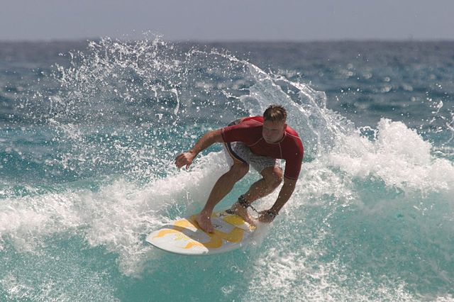
サーフィンしている男性（出典: wikimedia）

ここで使用されているモデルアーキテクチャは、「Show, Attend and Tell: Neural Image Caption Generation with Visual Attention」からアイデアを得たものですが、2 レイヤー Transformer デコーダを使用するように更新されています。このチュートリアルを最大限に活用するには、テキスト生成、seq2seq モデルとアテンション、または transformer の使用経験があるとよいでしょう。

以下は、このチュートリアルに組み込まれるモデルアーキテクチャです。特徴量は画像から抽出され、Transformer デコーダのクロスアテンションレイヤーに渡されています。

モデルアーキテクチャ

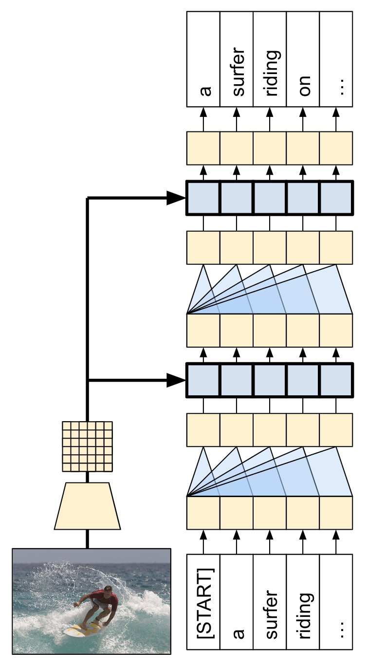
Transformer デコーダは主に、アテンションレイヤーから構築されます。セルフアテンションを使用して、生成されるシーケンスを処理し、クロスアテンションを使用して、画像に注意を向けます。

クロスアテンションレイヤーのアテンションの重みを検査することで、モデルが単語を生成する過程で、モデルが画像のどの部分を見ているかを知ることができます。

このノートブックは、エンドツーエンドの例を示します。このノートブックを実行すると、データセットのダウンロード、画像特徴量の抽出とキャッシュ処理、そしてデコーダモデルのトレーニングが行われます。その後で、モデルを使用して、新しい画像のキャプションが生成されるようになります。

セットアップ

!apt install --allow-change-held-packages libcudnn8=8.1.0.77-1+cuda11.2

!pip uninstall -y tensorflow estimator keras

!pip install -U tensorflow_text tensorflow tensorflow_datasets

!pip install einops

このチュートリアルでは多数の import を使用します。ほとんどがデータセットの読み込み目的です。

#@title
import concurrent.futures
import collections
import dataclasses
import hashlib
import itertools
import json
import math
import os
import pathlib
import random
import re
import string
import time
import urllib.request

import einops
import matplotlib.pyplot as plt
import numpy as np
import pandas as pd
from PIL import Image
import requests
import tqdm

import tensorflow as tf
import tensorflow_hub as hub
import tensorflow_text as text
import tensorflow_datasets as tfds

[オプション] データ処理

このセクションでは、captions データセットをダウンロードして、トレーニングの準備を行います。入力テキストをトークン化し、事前トレーニング済みの特徴量抽出器モデルを通じてすべての画像の実行結果をキャッシュします。このセクションの内容を完全に理解することは重要ではありません。

セクションをトグル

データセットを選択する

このチュートリアルは、データセットの選択肢を提供するようにセットアップされています。Flickr8k、または Conceptual Captions データセットの小さなスライスのいずれかを選択します。これらはゼロからダウンロードして変換されますが、TensorFlow Datasets で提供されている Coco Captions と完全な Conceptual Captions というキャプションデータセットを使用するようにチュートリアルを変更することは困難ではありません。

Flickr8k

def flickr8k(path='flickr8k'):
  path = pathlib.Path(path)

  if len(list(path.rglob('*'))) < 16197:
    tf.keras.utils.get_file(
        origin='https://github.com/jbrownlee/Datasets/releases/download/Flickr8k/Flickr8k_Dataset.zip',
        cache_dir='.',
        cache_subdir=path,
        extract=True)
    tf.keras.utils.get_file(
        origin='https://github.com/jbrownlee/Datasets/releases/download/Flickr8k/Flickr8k_text.zip',
        cache_dir='.',
        cache_subdir=path,
        extract=True)
    
  captions = (path/"Flickr8k.token.txt").read_text().splitlines()
  captions = (line.split('\t') for line in captions)
  captions = ((fname.split('#')[0], caption) for (fname, caption) in captions)

  cap_dict = collections.defaultdict(list)
  for fname, cap in captions:
    cap_dict[fname].append(cap)

  train_files = (path/'Flickr_8k.trainImages.txt').read_text().splitlines()
  train_captions = [(str(path/'Flicker8k_Dataset'/fname), cap_dict[fname]) for fname in train_files]

  test_files = (path/'Flickr_8k.testImages.txt').read_text().splitlines()
  test_captions = [(str(path/'Flicker8k_Dataset'/fname), cap_dict[fname]) for fname in test_files]

  train_ds = tf.data.experimental.from_list(train_captions)
  test_ds = tf.data.experimental.from_list(test_captions)

  return train_ds, test_ds

Conceptual Captions

def conceptual_captions(*, data_dir="conceptual_captions", num_train, num_val):
  def iter_index(index_path):
    with open(index_path) as f:
      for line in f:
        caption, url = line.strip().split('\t')
        yield caption, url

  def download_image_urls(data_dir, urls):
    ex = concurrent.futures.ThreadPoolExecutor(max_workers=100)
    def save_image(url):
      hash = hashlib.sha1(url.encode())
      # Name the files after the hash of the URL.
      file_path = data_dir/f'{hash.hexdigest()}.jpeg'
      if file_path.exists():
        # Only download each file once.
        return file_path

      try:
        result = requests.get(url, timeout=5)
      except Exception:
        file_path = None
      else:
        file_path.write_bytes(result.content)
      return file_path
    
    result = []
    out_paths = ex.map(save_image, urls)
    for file_path in tqdm.tqdm(out_paths, total=len(urls)):
      result.append(file_path)

    return result

  def ds_from_index_file(index_path, data_dir, count):
    data_dir.mkdir(exist_ok=True)
    index = list(itertools.islice(iter_index(index_path), count))
    captions = [caption for caption, url in index]
    urls = [url for caption, url in index]

    paths = download_image_urls(data_dir, urls)

    new_captions = []
    new_paths = []
    for cap, path in zip(captions, paths):
      if path is None:
        # Download failed, so skip this pair.
        continue
      new_captions.append(cap)
      new_paths.append(path)
    
    new_paths = [str(p) for p in new_paths]

    ds = tf.data.Dataset.from_tensor_slices((new_paths, new_captions))
    ds = ds.map(lambda path,cap: (path, cap[tf.newaxis])) # 1 caption per image
    return ds

  data_dir = pathlib.Path(data_dir)
  train_index_path = tf.keras.utils.get_file(
    origin='https://storage.googleapis.com/gcc-data/Train/GCC-training.tsv',
    cache_subdir=data_dir,
    cache_dir='.')
  
  val_index_path = tf.keras.utils.get_file(
    origin='https://storage.googleapis.com/gcc-data/Validation/GCC-1.1.0-Validation.tsv',
    cache_subdir=data_dir,
    cache_dir='.')
  
  train_raw = ds_from_index_file(train_index_path, data_dir=data_dir/'train', count=num_train)
  test_raw = ds_from_index_file(val_index_path, data_dir=data_dir/'val', count=num_val)

  return train_raw, test_raw

データセットをダウンロードする

Flickr8k には 1 つの画像につき 5 つのキャプションが含まれているため、より小さなダウンロードサイズでより多くのデータを得られる良い選択肢と言えます。

choose = 'flickr8k'

if choose == 'flickr8k':
  train_raw, test_raw = flickr8k()
else:
  train_raw, test_raw = conceptual_captions(num_train=10000, num_val=5000)

上記のいずれのデータセットのローダーも、(image_path, captions) ペアを含む tf.data.Dataset を返します。Flickr8k データセットには 1 つの画像につき 5 つのキャプションが含まれているのに対し、Conceptual Captions のキャプションは 1 つです。

train_raw.element_spec

for ex_path, ex_captions in train_raw.take(1):
  print(ex_path)
  print(ex_captions)

画像特徴量抽出器

画像モデル（imagenet で事前トレーニング済み）を使用して各画像から特徴量を抽出します。このモデルは画像分類器としてトレーニングされていますが、設定 include_top=False は最終的な分類レイヤーなしのモデルを返すため、特徴量マップの最後のレイヤーを使用できます。

IMAGE_SHAPE=(224, 224, 3)
mobilenet = tf.keras.applications.MobileNetV3Small(
    input_shape=IMAGE_SHAPE,
    include_top=False,
    include_preprocessing=True)
mobilenet.trainable=False

以下は、画像を読み込んでモデルに合わせてサイズを変更する関数です。

def load_image(image_path):
    img = tf.io.read_file(image_path)
    img = tf.io.decode_jpeg(img, channels=3)
    img = tf.image.resize(img, IMAGE_SHAPE[:-1])
    return img

モデルは、入力バッチで各画像の特徴量マップを返します。

test_img_batch = load_image(ex_path)[tf.newaxis, :]

print(test_img_batch.shape)
print(mobilenet(test_img_batch).shape)

テキストトークナイザ/ベクタナイザをセットアップする

次の手順で、TextVectorization レイヤーを使用して、テキストキャプションを整数シーケンスに変換します。

• adapt を使用して、すべてのキャプションをイテレートし、キャプションを単語に分割して、上位の単語の語彙を計算します。

• 各単語を語彙のインデックスにマッピングして、すべてのキャプションをトークン化します。すべての出力シーケンスは、長さ 50 までパディングされます。

• 結果を表示するために、単語からインデックスおよびインデックスから単語へのマッピングを作成します。

def standardize(s):
  s = tf.strings.lower(s)
  s = tf.strings.regex_replace(s, f'[{re.escape(string.punctuation)}]', '')
  s = tf.strings.join(['[START]', s, '[END]'], separator=' ')
  return s

# Use the top 5000 words for a vocabulary.
vocabulary_size = 5000
tokenizer = tf.keras.layers.TextVectorization(
    max_tokens=vocabulary_size,
    standardize=standardize,
    ragged=True)
# Learn the vocabulary from the caption data.

tokenizer.adapt(train_raw.map(lambda fp,txt: txt).unbatch().batch(1024))

tokenizer.get_vocabulary()[:10]

t = tokenizer([['a cat in a hat'], ['a robot dog']])
t

# Create mappings for words to indices and indices to words.
word_to_index = tf.keras.layers.StringLookup(
    mask_token="",
    vocabulary=tokenizer.get_vocabulary())
index_to_word = tf.keras.layers.StringLookup(
    mask_token="",
    vocabulary=tokenizer.get_vocabulary(),
    invert=True)

w = index_to_word(t)
w.to_list()

tf.strings.reduce_join(w, separator=' ', axis=-1).numpy()

データセットを準備する

train_raw と test_raw データセットには、一対多の (image, captions) ペアが含まれます。

この関数は、画像とキャプションが 1:1 になるように、画像を複製します。

def match_shapes(images, captions):
  caption_shape = einops.parse_shape(captions, 'b c')
  captions = einops.rearrange(captions, 'b c -> (b c)')
  images = einops.repeat(
      images, 'b ... -> (b c) ...',
      c = caption_shape['c'])
  return images, captions

for ex_paths, ex_captions in train_raw.batch(32).take(1):
  break

print('image paths:', ex_paths.shape)
print('captions:', ex_captions.shape)
print()

ex_paths, ex_captions = match_shapes(images=ex_paths, captions=ex_captions)

print('image_paths:', ex_paths.shape)
print('captions:', ex_captions.shape)

Keras トレーニングと互換性を持たせるため、データセットには (inputs, labels) ペアを含める必要があります。テキスト生成では、トークンは、入力とラベルのいずれでもあり、1 ステップずつシフトされます。この関数は、(images, texts) ペアを ((images, input_tokens), label_tokens) ペアに変換します。

def prepare_txt(imgs, txts):
  tokens = tokenizer(txts)

  input_tokens = tokens[..., :-1]
  label_tokens = tokens[..., 1:]
  return (imgs, input_tokens), label_tokens

この関数は、以下の手順でデータセットに演算を追加します。

1. 画像を読み込みます（読み込みに失敗する画像は無視されます）。

2. キャプションの数に合わせて画像を複製します。

3. image, caption ペアをシャッフルして再バッチ化します。

4. テキストをトークン化し、トークンをシフトして label_tokens を追加します。

5. RaggedTensor 表現のテキストをパディング付きの高密度 Tensor 表現に変換します。

def prepare_dataset(ds, tokenizer, batch_size=32, shuffle_buffer=1000):
  # Load the images and make batches.
  ds = (ds
        .shuffle(10000)
        .map(lambda path, caption: (load_image(path), caption))
        .apply(tf.data.experimental.ignore_errors())
        .batch(batch_size))

  def to_tensor(inputs, labels):
    (images, in_tok), out_tok = inputs, labels
    return (images, in_tok.to_tensor()), out_tok.to_tensor()

  return (ds
          .map(match_shapes, tf.data.AUTOTUNE)
          .unbatch()
          .shuffle(shuffle_buffer)
          .batch(batch_size)
          .map(prepare_txt, tf.data.AUTOTUNE)
          .map(to_tensor, tf.data.AUTOTUNE)
          )

以下のようにして、特徴量抽出器をモデルにインストールし、データセットでトレーニングすることが可能です。

train_ds = prepare_dataset(train_raw, tokenizer)
train_ds.element_spec

test_ds = prepare_dataset(test_raw, tokenizer)
test_ds.element_spec

[オプション] 画像特徴量をキャッシュする

画像特徴量抽出器には変化がなく、このチュートリアルでは画像拡張を使用していないため、画像特徴量をキャッシュすることができます。テキストトークン化についても同様です。キャッシュをセットアップするのに時間がかかりますが、その時間は、トレーニングと検証中に、各エポックで取り返すことができます。以下のコードでは、save_dataset と load_dataset の 2 つの関数を定義しています。

def save_dataset(ds, save_path, image_model, tokenizer, shards=10, batch_size=32):
  # Load the images and make batches.
  ds = (ds
        .map(lambda path, caption: (load_image(path), caption))
        .apply(tf.data.experimental.ignore_errors())
        .batch(batch_size))

  # Run the feature extractor on each batch
  # Don't do this in a .map, because tf.data runs on the CPU. 
  def gen():
    for (images, captions) in tqdm.tqdm(ds): 
      feature_maps = image_model(images)

      feature_maps, captions = match_shapes(feature_maps, captions)
      yield feature_maps, captions

  # Wrap the generator in a new tf.data.Dataset.
  new_ds = tf.data.Dataset.from_generator(
      gen,
      output_signature=(
          tf.TensorSpec(shape=image_model.output_shape),
          tf.TensorSpec(shape=(None,), dtype=tf.string)))

  # Apply the tokenization 
  new_ds = (new_ds
            .map(prepare_txt, tf.data.AUTOTUNE)
            .unbatch()
            .shuffle(1000))

  # Save the dataset into shard files.
  def shard_func(i, item):
    return i % shards
  new_ds.enumerate().save(save_path, shard_func=shard_func)

def load_dataset(save_path, batch_size=32, shuffle=1000, cycle_length=2):
  def custom_reader_func(datasets):
    datasets = datasets.shuffle(1000)
    return datasets.interleave(lambda x: x, cycle_length=cycle_length)
  
  ds = tf.data.Dataset.load(save_path, reader_func=custom_reader_func)

  def drop_index(i, x):
    return x

  ds = (ds
        .map(drop_index, tf.data.AUTOTUNE)
        .shuffle(shuffle)
        .padded_batch(batch_size)
        .prefetch(tf.data.AUTOTUNE))
  return ds

save_dataset(train_raw, 'train_cache', mobilenet, tokenizer)
save_dataset(test_raw, 'test_cache', mobilenet, tokenizer)

トレーニングの準備が完了したデータ

前処理手順が完了したら、データセットは以下のようになります。

train_ds = load_dataset('train_cache')
test_ds = load_dataset('test_cache')

train_ds.element_spec

このデータセットは、Keras でのトレーニングに適した (input, label) ペアを返すようになりました。inputs は (images, input_tokens) ペアです。images は特徴量抽出器モデルで処理が完了しています。input_tokens の各場所では、モデルはそれまでのテキストを見て、labels 内の同じ位置に並んでいる次のテキストを予測しようとします。

for (inputs, ex_labels) in train_ds.take(1):
  (ex_img, ex_in_tok) = inputs

print(ex_img.shape)
print(ex_in_tok.shape)
print(ex_labels.shape)

入力トークンとラベルは、1 ステップずつシフトしているだけで、同じです。

print(ex_in_tok[0].numpy())
print(ex_labels[0].numpy())

Transformer デコーダモデル

このモデルは、事前トレーニング済みの画像エンコーダが十分であることを前提としているため、テキストエンコーダの構築のみに焦点を当てています。このチュートリアルでは 2 レイヤーの Transformer デコーダを使用します。

実装は、Transformers チュートリアルとほぼ同一です。詳細は、そちらをご覧ください。

Transformer エンコーダとデコーダ

モデルは、主に以下の 3 つのパーツで実装されます。

1. 入力 - トークン埋め込みと位置エンコーディング（SeqEmbedding）。

2. デコーダ - Transformer デコーダレイヤーのスタック（DecoderLayer）で、それぞれに以下が含まれます。

   1. カジュアルなセルフアテンションレイヤー（CausalSelfAttention）。出力の各場所はそれまでの出力に注目します。

   2. クロスアテンションレイヤー（CrossAttention）。出力の各場所は入力画像に注目します。

   3. フィードフォワードネットワーク（FeedForward）レイヤー。各出力場所をさらに個別に処理します。

3. 出力 - 出力語彙に対するマルチクラス分類。

入力

入力テキストはすでにトークンに分割され、ID のシーケンスに変換されています。

CNN や RNN とは異なり、Transformer のアテンションレイヤーは、シーケンスの順序に対して不変であることを思い出しましょう。なんらかの位置入力がないと、シーケンスではなく順序付けられていないセットが表示されます。そのため、Embedding レイヤーには、各トークンの単純なベクトル埋め込みの他に、シーケンスの各位置の埋め込みも含められます。

SeqEmbedding レイヤーは以下のように定義されています。

• 各トークンの埋め込みベクトルをルックアップします。

• 各シーケンス位置の埋め込みベクトルをルックアップします。

• その両方を追加します。

• mask_zero=True を使用して、モデルの keras-masks を初期化します。

注意: この実装は、Transformer チュートリアルのように固定埋め込みを使用する代わりに、位置埋め込みを学習します。埋め込みの学習ではコードがわずかに少なくなりますが、より長いシーケンスには一般化されません。

class SeqEmbedding(tf.keras.layers.Layer):
  def __init__(self, vocab_size, max_length, depth):
    super().__init__()
    self.pos_embedding = tf.keras.layers.Embedding(input_dim=max_length, output_dim=depth)

    self.token_embedding = tf.keras.layers.Embedding(
        input_dim=vocab_size,
        output_dim=depth,
        mask_zero=True)
    
    self.add = tf.keras.layers.Add()

  def call(self, seq):
    seq = self.token_embedding(seq) # (batch, seq, depth)

    x = tf.range(tf.shape(seq)[1])  # (seq)
    x = x[tf.newaxis, :]  # (1, seq)
    x = self.pos_embedding(x)  # (1, seq, depth)

    return self.add([seq,x])

デコーダ

デコーダは標準的な Transformer デコーダで、それぞれに CausalSelfAttention、CrossAttention、および FeedForward-decoder の 3 つのサブレイヤーを含む DecoderLayers のスタックが含まれます。実装は Transformer チュートリアルとほぼ同一であるため、詳細はそちらをご覧ください。

以下は、CausalSelfAttention レイヤーです。

class CausalSelfAttention(tf.keras.layers.Layer):
  def __init__(self, **kwargs):
    super().__init__()
    self.mha = tf.keras.layers.MultiHeadAttention(**kwargs)
    # Use Add instead of + so the keras mask propagates through.
    self.add = tf.keras.layers.Add() 
    self.layernorm = tf.keras.layers.LayerNormalization()
  
  def call(self, x):
    attn = self.mha(query=x, value=x,
                    use_causal_mask=True)
    x = self.add([x, attn])
    return self.layernorm(x)

以下は、CrossAttention レイヤーです。return_attention_scores の使用に注意してください。

class CrossAttention(tf.keras.layers.Layer):
  def __init__(self,**kwargs):
    super().__init__()
    self.mha = tf.keras.layers.MultiHeadAttention(**kwargs)
    self.add = tf.keras.layers.Add() 
    self.layernorm = tf.keras.layers.LayerNormalization()
  
  def call(self, x, y, **kwargs):
    attn, attention_scores = self.mha(
             query=x, value=y,
             return_attention_scores=True)
    
    self.last_attention_scores = attention_scores

    x = self.add([x, attn])
    return self.layernorm(x)

以下は、FeedForward レイヤーです。layers.Dense レイヤーは入力の最後の軸に適用されることを思い出しましょう。入力は (batch, sequence, channels) の形状になるため、batch と sequence 軸にポイントワイズが自動的に適用されます。

class FeedForward(tf.keras.layers.Layer):
  def __init__(self, units, dropout_rate=0.1):
    super().__init__()
    self.seq = tf.keras.Sequential([
        tf.keras.layers.Dense(units=2*units, activation='relu'),
        tf.keras.layers.Dense(units=units),
        tf.keras.layers.Dropout(rate=dropout_rate),
    ])

    self.layernorm = tf.keras.layers.LayerNormalization()
  
  def call(self, x):
    x = x + self.seq(x)
    return self.layernorm(x)

次に、これらの 3 つのレイヤーをより大きな DecoderLayer に配置します。各デコーダレイヤーは、3 つの小さなレイヤーをシーケンスで適用します。各サブレイヤーの後、out_seq の形状は (batch, sequence, channels) になります。デコーダレイヤーは、後で可視化できる attention_scores も返します。

class DecoderLayer(tf.keras.layers.Layer):
  def __init__(self, units, num_heads=1, dropout_rate=0.1):
    super().__init__()
    
    self.self_attention = CausalSelfAttention(num_heads=num_heads,
                                              key_dim=units,
                                              dropout=dropout_rate)
    self.cross_attention = CrossAttention(num_heads=num_heads,
                                          key_dim=units,
                                          dropout=dropout_rate)
    self.ff = FeedForward(units=units, dropout_rate=dropout_rate)
      

  def call(self, inputs, training=False):
    in_seq, out_seq = inputs

    # Text input
    out_seq = self.self_attention(out_seq)

    out_seq = self.cross_attention(out_seq, in_seq)
    
    self.last_attention_scores = self.cross_attention.last_attention_scores

    out_seq = self.ff(out_seq)

    return out_seq

出力

最低でも、出力レイヤーには、各位置で各トークンのロジット予測を生成するための layers.Dense レイヤーが必要です。

しかし、この動作を少しでも改良するために追加できる他の特徴量は少ししかありません。

1. 不正なトークンを処理する: モデルはテキストを生成します。パディング、不明、または開始トークン（''、'[UNK]'、'[START]'）を絶対に生成してはいけません。したがって、これらのバイアスは大きな負の値に設定します。

   注意: これらのトークンは、損失関数ででも無視する必要があります。

2. スマート初期化: 高密度レイヤーのデフォルトの初期化では、最初にほぼ一様の尤度で各トークンを予測するモデルが得られます。実際のトークン分布は一様からはほど遠いものです。出力レイヤーの初期バイアスの最適な値は、各トークンの確率の対数です。したがって、adapt メソッドを含めてトークンをカウントし、最適な初期バイアスを設定します。こうすることで、初期損失が一様分布のエントロピー（log(vocabulary_size)）から分布の限界エントロピー（-p*log(p)）に減少します。

#@title
class TokenOutput(tf.keras.layers.Layer):
  def __init__(self, tokenizer, banned_tokens=('', '[UNK]', '[START]'), **kwargs):
    super().__init__()
    
    self.dense = tf.keras.layers.Dense(
        units=tokenizer.vocabulary_size(), **kwargs)
    self.tokenizer = tokenizer
    self.banned_tokens = banned_tokens

    self.bias = None

  def adapt(self, ds):
    counts = collections.Counter()
    vocab_dict = {name: id 
                  for id, name in enumerate(self.tokenizer.get_vocabulary())}

    for tokens in tqdm.tqdm(ds):
      counts.update(tokens.numpy().flatten())

    counts_arr = np.zeros(shape=(self.tokenizer.vocabulary_size(),))
    counts_arr[np.array(list(counts.keys()), dtype=np.int32)] = list(counts.values())

    counts_arr = counts_arr[:]
    for token in self.banned_tokens:
      counts_arr[vocab_dict[token]] = 0

    total = counts_arr.sum()
    p = counts_arr/total
    p[counts_arr==0] = 1.0
    log_p = np.log(p)  # log(1) == 0

    entropy = -(log_p*p).sum()

    print()
    print(f"Uniform entropy: {np.log(self.tokenizer.vocabulary_size()):0.2f}")
    print(f"Marginal entropy: {entropy:0.2f}")

    self.bias = log_p
    self.bias[counts_arr==0] = -1e9

  def call(self, x):
    x = self.dense(x)
    # TODO(b/250038731): Fix this.
    # An Add layer doesn't work because of the different shapes.
    # This clears the mask, that's okay because it prevents keras from rescaling
    # the losses.
    return x + self.bias

スマート初期化によって、初期損失をが大幅に減少します。

output_layer = TokenOutput(tokenizer, banned_tokens=('', '[UNK]', '[START]'))
# This might run a little faster if the dataset didn't also have to load the image data.
output_layer.adapt(train_ds.map(lambda inputs, labels: labels))

モデルを構築する

モデルを構築するには、複数のパーツを組み合わせる必要があります。

1. 画像 feature_extractor とテキスト tokenizer。

2. seq_embedding レイヤー。トークン ID のバッチをベクトル (batch, sequence, channels) に変換します。

3. テキストと画像データを処理する DecoderLayers レイヤーのスタック。

4. output_layer。次の単語のポイントワイズの予測を返します。

class Captioner(tf.keras.Model):
  @classmethod
  def add_method(cls, fun):
    setattr(cls, fun.__name__, fun)
    return fun

  def __init__(self, tokenizer, feature_extractor, output_layer, num_layers=1,
               units=256, max_length=50, num_heads=1, dropout_rate=0.1):
    super().__init__()
    self.feature_extractor = feature_extractor
    self.tokenizer = tokenizer
    self.word_to_index = tf.keras.layers.StringLookup(
        mask_token="",
        vocabulary=tokenizer.get_vocabulary())
    self.index_to_word = tf.keras.layers.StringLookup(
        mask_token="",
        vocabulary=tokenizer.get_vocabulary(),
        invert=True) 

    self.seq_embedding = SeqEmbedding(
        vocab_size=tokenizer.vocabulary_size(),
        depth=units,
        max_length=max_length)

    self.decoder_layers = [
        DecoderLayer(units, num_heads=num_heads, dropout_rate=dropout_rate)
        for n in range(num_layers)]

    self.output_layer = output_layer

トレーニングにモデルを呼び出すと、image, txt ペアが返されます。この関数をさらに使いやすくするために、入力について柔軟になりましょう。

• 画像に 3 つのチャンネルがある場合、feature_extractor に通します。そうでない場合は、すでに通過済みであることを前提とします。

• テキストに dtype tf.string がある場合、tokenizer に通します。

その後のモデルの実行はほんの数ステップです。

1. 抽出された画像特徴量をフラット化し、デコーダレイヤーに入力できるようにします。

2. トークン埋め込みをルックアップします。

3. 画像特徴量とテキスト埋め込みで DecoderLayer を実行します。

4. 出力レイヤーを実行して、各位置の次のトークンを予測します。

  @Captioner.add_method
  def call(self, inputs):
    image, txt = inputs

    if image.shape[-1] == 3:
      # Apply the feature-extractor, if you get an RGB image.
      image = self.feature_extractor(image)
    
    # Flatten the feature map
    image = einops.rearrange(image, 'b h w c -> b (h w) c')


    if txt.dtype == tf.string:
      # Apply the tokenizer if you get string inputs.
      txt = tokenizer(txt)

    txt = self.seq_embedding(txt)

    # Look at the image
    for dec_layer in self.decoder_layers:
      txt = dec_layer(inputs=(image, txt))
      
    txt = self.output_layer(txt)

    return txt

model = Captioner(tokenizer, feature_extractor=mobilenet, output_layer=output_layer,
                  units=256, dropout_rate=0.5, num_layers=2, num_heads=2)

キャプションを生成する

トレーニングに進む前に、キャプションを生成するコードを記述します。これを使用して、トレーニングの進捗状況を確認します。

テスト画像のダウンロードから始めましょう。

image_url = 'https://tensorflow.org/images/surf.jpg'
image_path = tf.keras.utils.get_file('surf.jpg', origin=image_url)
image = load_image(image_path)

このモデルで画像にキャプションを付けるには、以下のようにします。

• img_features を抽出します。

• [START] トークンで出力トークンのリストを初期化します。

• img_features と tokens をモデルに渡します。

  • ロジットのリストが返されます。

  • これらのロジットに基づいて、次のトークンを選択します。

  • それをトークンのリストに追加し、ループを続けます。

  • '[END]' トークンが生成されたら、ループを抜けます。

では、これを行うだけの「単純な」メソッドを追加しましょう。

@Captioner.add_method
def simple_gen(self, image, temperature=1):
  initial = self.word_to_index([['[START]']]) # (batch, sequence)
  img_features = self.feature_extractor(image[tf.newaxis, ...])

  tokens = initial # (batch, sequence)
  for n in range(50):
    preds = self((img_features, tokens)).numpy()  # (batch, sequence, vocab)
    preds = preds[:,-1, :]  #(batch, vocab)
    if temperature==0:
        next = tf.argmax(preds, axis=-1)[:, tf.newaxis]  # (batch, 1)
    else:
        next = tf.random.categorical(preds/temperature, num_samples=1)  # (batch, 1)
    tokens = tf.concat([tokens, next], axis=1) # (batch, sequence) 

    if next[0] == self.word_to_index('[END]'):
      break
  words = index_to_word(tokens[0, 1:-1])
  result = tf.strings.reduce_join(words, axis=-1, separator=' ')
  return result.numpy().decode()

以下は、その画像に生成されたいくつかのキャプションです。モデルはトレーニングされていないため、まだあまり意味を成しません。

for t in (0.0, 0.5, 1.0):
  result = model.simple_gen(image, temperature=t)
  print(result)

temperature パラメータを使うと、3 つのモード間を補間できます。

1. Greedy デコーディング（temperature=0.0）- 各ステップで最も可能性の高い次のトークンを選択します。

2. ロジットに基づくランダムサンプリング（temperature=1.0）。

3. 一様のランダムサンプリング（temperature >> 1.0）。

モデルはトレーニングされていないため、また頻度ベースの初期化を使用しているため、"greedy" 出力（最初の出力）には通常、最も一般的なトークン tokens: ['a', '.', '[END]'] のみが含まれます。

トレーニング

モデルをトレーニングするには、追加コンポーネントがいくつか必要となります。

• 損失と指標

• オプティマイザ

• オプションのコールバック

損失と指標

以下は、マスクされた損失と精度の実装です。

損失のマスクを計算する際は、loss < 1e8 に注意してください。この項は、banned_tokens の人為的で、ありえないほど大きな損失を破棄します。

def masked_loss(labels, preds):  
  loss = tf.nn.sparse_softmax_cross_entropy_with_logits(labels, preds)

  mask = (labels != 0) & (loss < 1e8) 
  mask = tf.cast(mask, loss.dtype)

  loss = loss*mask
  loss = tf.reduce_sum(loss)/tf.reduce_sum(mask)
  return loss

def masked_acc(labels, preds):
  mask = tf.cast(labels!=0, tf.float32)
  preds = tf.argmax(preds, axis=-1)
  labels = tf.cast(labels, tf.int64)
  match = tf.cast(preds == labels, mask.dtype)
  acc = tf.reduce_sum(match*mask)/tf.reduce_sum(mask)
  return acc

コールバック

トレーニング中のフィードバックでは、keras.callbacks.Callback を、サーファーの画像のキャプションを各エポックの最後に生成するようにセットアップします。

class GenerateText(tf.keras.callbacks.Callback):
  def __init__(self):
    image_url = 'https://tensorflow.org/images/surf.jpg'
    image_path = tf.keras.utils.get_file('surf.jpg', origin=image_url)
    self.image = load_image(image_path)

  def on_epoch_end(self, epochs=None, logs=None):
    print()
    print()
    for t in (0.0, 0.5, 1.0):
      result = self.model.simple_gen(self.image, temperature=t)
      print(result)
    print()

これは、前の例のような 3 つの出力文字列を生成します。前と同様に、最初に「greedy」を使用し、各ステップでロジットの argmax を選択します。

g = GenerateText()
g.model = model
g.on_epoch_end(0)

また、callbacks.EarlyStopping を使用して、モデルが過学習し始めたらトレーニングを終了するようにします。

callbacks = [
    GenerateText(),
    tf.keras.callbacks.EarlyStopping(
        patience=5, restore_best_weights=True)]

トレーニング

トレーニングを構成して実行します。

model.compile(optimizer=tf.keras.optimizers.Adam(learning_rate=1e-4),
           loss=masked_loss,
           metrics=[masked_acc])

より頻繁にレポートするには、Dataset.repeat() メソッドを使用し、steps_per_epoch と validation_steps 引数を Model.fit に設定します。

Flickr8k でこのようにセットアップすると、データセット全体の完全なパスは 900 以上のバッチですが、レポートエポックより下は 100 ステップとなります。

history = model.fit(
    train_ds.repeat(),
    steps_per_epoch=100,
    validation_data=test_ds.repeat(),
    validation_steps=20,
    epochs=100,
    callbacks=callbacks)

トレーニングランの損失と精度をプロットします。

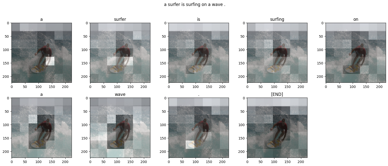
plt.plot(history.history['loss'], label='loss')
plt.plot(history.history['val_loss'], label='val_loss')
plt.ylim([0, max(plt.ylim())])
plt.xlabel('Epoch #')
plt.ylabel('CE/token')
plt.legend()

plt.plot(history.history['masked_acc'], label='accuracy')
plt.plot(history.history['val_masked_acc'], label='val_accuracy')
plt.ylim([0, max(plt.ylim())])
plt.xlabel('Epoch #')
plt.ylabel('CE/token')
plt.legend()

アテンションプロット

次に、トレーニング済みのモデルを使用して、画像に simple_gen メソッドを実行します。

result = model.simple_gen(image, temperature=0.0)
result

出力をトークンに分割し直します。

str_tokens = result.split()
str_tokens.append('[END]')

DecoderLayers はそれぞれ、CrossAttention レイヤーのアテンションスコアをキャッシュします。各アテンションマップの形状は (batch=1, heads, sequence, image) です。

attn_maps = [layer.last_attention_scores for layer in model.decoder_layers]
[map.shape for map in attn_maps]

したがって、batch 軸に沿ってマップをスタックし、(batch, heads) 軸で平均しながら、image 軸を height, width に分割し直します。

attention_maps = tf.concat(attn_maps, axis=0)
attention_maps = einops.reduce(
    attention_maps,
    'batch heads sequence (height width) -> sequence height width',
    height=7, width=7,
    reduction='mean')

シーケンス予測ごとに、多につのアテンションマップを得られました。各マップの値の和は 1 になります。

einops.reduce(attention_maps, 'sequence height width -> sequence', reduction='sum')

したがって、出力の各トークンを生成する際にモデルが注意を向けていた場所は以下です。

def plot_attention_maps(image, str_tokens, attention_map):
    fig = plt.figure(figsize=(16, 9))

    len_result = len(str_tokens)
    
    titles = []
    for i in range(len_result):
      map = attention_map[i]
      grid_size = max(int(np.ceil(len_result/2)), 2)
      ax = fig.add_subplot(3, grid_size, i+1)
      titles.append(ax.set_title(str_tokens[i]))
      img = ax.imshow(image)
      ax.imshow(map, cmap='gray', alpha=0.6, extent=img.get_extent(),
                clim=[0.0, np.max(map)])

    plt.tight_layout()

plot_attention_maps(image/255, str_tokens, attention_maps)

次に、これをより使いやすい関数にまとめます。

@Captioner.add_method
def run_and_show_attention(self, image, temperature=0.0):
  result_txt = self.simple_gen(image, temperature)
  str_tokens = result_txt.split()
  str_tokens.append('[END]')

  attention_maps = [layer.last_attention_scores for layer in self.decoder_layers]
  attention_maps = tf.concat(attention_maps, axis=0)
  attention_maps = einops.reduce(
      attention_maps,
      'batch heads sequence (height width) -> sequence height width',
      height=7, width=7,
      reduction='mean')
  
  plot_attention_maps(image/255, str_tokens, attention_maps)
  t = plt.suptitle(result_txt)
  t.set_y(1.05)

run_and_show_attention(model, image)

あなた独自の画像でためそう

トレーニングしたばかりのモデルで独自の画像にキャプションを付ける方法を以下に示します。比較的少量のデータでトレーニングされているので、使用する画像がトレーニングデータと異なることがあることに注意してください（奇妙な結果がでるかもしれません！）

image_url = 'https://tensorflow.org/images/bedroom_hrnet_tutorial.jpg'
image_path = tf.keras.utils.get_file(origin=image_url)
image = load_image(image_path)

run_and_show_attention(model, image)