video_classification.ipynb

Kernel: Python 3

Copyright 2022 The TensorFlow Authors.

#@title Licensed under the Apache License, Version 2.0 (the "License");
# you may not use this file except in compliance with the License.
# You may obtain a copy of the License at
#
# https://www.apache.org/licenses/LICENSE-2.0
#
# Unless required by applicable law or agreed to in writing, software
# distributed under the License is distributed on an "AS IS" BASIS,
# WITHOUT WARRANTIES OR CONDITIONS OF ANY KIND, either express or implied.
# See the License for the specific language governing permissions and
# limitations under the License.

TensorFlow.org에서 보기

Google Colab에서 실행하기

GitHub에서 소스 보기

노트북 다운로드하기

3D 컨볼루셔널 신경망을 사용한 비디오 분류

This tutorial demonstrates training a 3D convolutional neural network (CNN) for video classification using the UCF101 action recognition dataset. A 3D CNN uses a three-dimensional filter to perform convolutions. The kernel is able to slide in three directions, whereas in a 2D CNN it can slide in two dimensions. The model is based on the work published in A Closer Look at Spatiotemporal Convolutions for Action Recognition by D. Tran et al. (2017). In this tutorial, you will:

• 입력 파이프라인을 구축합니다.

• Keras 함수형 API를 사용하여 잔차 연결이 있는 3D 컨볼루셔널 신경망 모델을 구축합니다.

• 모델 학습

• 모델을 평가 및 테스트합니다.

This video classification tutorial is the second part in a series of TensorFlow video tutorials. Here are the other three tutorials:

• Load video data: This tutorial explains much of the code used in this document.

• MoViNet for streaming action recognition: Get familiar with the MoViNet models that are available on TF Hub.

• Transfer learning for video classification with MoViNet: This tutorial explains how to use a pre-trained video classification model trained on a different dataset with the UCF-101 dataset.

설정

먼저 ZIP 파일의 내용을 검사하기 위한 remotezip, 진행률 표시줄을 사용하기 위한 tqdm, 비디오 파일을 처리하기 위한 OpenCV, 더 복잡한 텐서 작업을 수행하기 위한 einops, Jupyter 노트북에 데이터를 내장하기 위한 tensorflow_docs 등 일부 필요한 라이브러리를 설치하고 가져옵니다.

Note: Use TensorFlow 2.10 to run this tutorial. Versions above TensorFlow 2.10 may not run successfully.

!pip install remotezip tqdm opencv-python einops

import tqdm
import random
import pathlib
import itertools
import collections

import cv2
import einops
import numpy as np
import remotezip as rz
import seaborn as sns
import matplotlib.pyplot as plt

import tensorflow as tf
import keras
from keras import layers

비디오 데이터 로드 및 전처리

아래 숨겨진 셀은 UCF-101 데이터세트에서 데이터 조각을 다운로드하고 tf.data.Dataset에 로드하는 헬퍼 함수를 정의합니다. 이 코드를 자세히 안내하는 비디오 데이터 로드 튜토리얼에서 특정 전처리 단계에 대해 자세히 알아볼 수 있습니다.

숨겨진 블록 끝에 있는 FrameGenerator 클래스는 여기에서 가장 중요한 유틸리티로, TensorFlow 데이터 파이프라인에 데이터를 공급할 수 있는 반복 가능한 객체를 생성합니다. 특히 이 클래스에는 인코딩된 레이블과 함께 비디오 프레임을 로드하는 Python 생성기가 포함되어 있습니다. 생성기(__call__) 함수는 frames_from_video_file에 의해 생성된 프레임 배열과 프레임 세트와 관련된 레이블의 원-핫 인코딩 벡터를 생성합니다.

#@title

def list_files_per_class(zip_url):
  """
    List the files in each class of the dataset given the zip URL.

    Args:
      zip_url: URL from which the files can be unzipped. 

    Return:
      files: List of files in each of the classes.
  """
  files = []
  with rz.RemoteZip(URL) as zip:
    for zip_info in zip.infolist():
      files.append(zip_info.filename)
  return files

def get_class(fname):
  """
    Retrieve the name of the class given a filename.

    Args:
      fname: Name of the file in the UCF101 dataset.

    Return:
      Class that the file belongs to.
  """
  return fname.split('_')[-3]

def get_files_per_class(files):
  """
    Retrieve the files that belong to each class. 

    Args:
      files: List of files in the dataset.

    Return:
      Dictionary of class names (key) and files (values).
  """
  files_for_class = collections.defaultdict(list)
  for fname in files:
    class_name = get_class(fname)
    files_for_class[class_name].append(fname)
  return files_for_class

def download_from_zip(zip_url, to_dir, file_names):
  """
    Download the contents of the zip file from the zip URL.

    Args:
      zip_url: Zip URL containing data.
      to_dir: Directory to download data to.
      file_names: Names of files to download.
  """
  with rz.RemoteZip(zip_url) as zip:
    for fn in tqdm.tqdm(file_names):
      class_name = get_class(fn)
      zip.extract(fn, str(to_dir / class_name))
      unzipped_file = to_dir / class_name / fn

      fn = pathlib.Path(fn).parts[-1]
      output_file = to_dir / class_name / fn
      unzipped_file.rename(output_file,)

def split_class_lists(files_for_class, count):
  """
    Returns the list of files belonging to a subset of data as well as the remainder of
    files that need to be downloaded.
    
    Args:
      files_for_class: Files belonging to a particular class of data.
      count: Number of files to download.

    Return:
      split_files: Files belonging to the subset of data.
      remainder: Dictionary of the remainder of files that need to be downloaded.
  """
  split_files = []
  remainder = {}
  for cls in files_for_class:
    split_files.extend(files_for_class[cls][:count])
    remainder[cls] = files_for_class[cls][count:]
  return split_files, remainder

def download_ufc_101_subset(zip_url, num_classes, splits, download_dir):
  """
    Download a subset of the UFC101 dataset and split them into various parts, such as
    training, validation, and test. 

    Args:
      zip_url: Zip URL containing data.
      num_classes: Number of labels.
      splits: Dictionary specifying the training, validation, test, etc. (key) division of data 
              (value is number of files per split).
      download_dir: Directory to download data to.

    Return:
      dir: Posix path of the resulting directories containing the splits of data.
  """
  files = list_files_per_class(zip_url)
  for f in files:
    tokens = f.split('/')
    if len(tokens) <= 2:
      files.remove(f) # Remove that item from the list if it does not have a filename
  
  files_for_class = get_files_per_class(files)

  classes = list(files_for_class.keys())[:num_classes]

  for cls in classes:
    new_files_for_class = files_for_class[cls]
    random.shuffle(new_files_for_class)
    files_for_class[cls] = new_files_for_class
    
  # Only use the number of classes you want in the dictionary
  files_for_class = {x: files_for_class[x] for x in list(files_for_class)[:num_classes]}

  dirs = {}
  for split_name, split_count in splits.items():
    print(split_name, ":")
    split_dir = download_dir / split_name
    split_files, files_for_class = split_class_lists(files_for_class, split_count)
    download_from_zip(zip_url, split_dir, split_files)
    dirs[split_name] = split_dir

  return dirs

def format_frames(frame, output_size):
  """
    Pad and resize an image from a video.
    
    Args:
      frame: Image that needs to resized and padded. 
      output_size: Pixel size of the output frame image.

    Return:
      Formatted frame with padding of specified output size.
  """
  frame = tf.image.convert_image_dtype(frame, tf.float32)
  frame = tf.image.resize_with_pad(frame, *output_size)
  return frame

def frames_from_video_file(video_path, n_frames, output_size = (224,224), frame_step = 15):
  """
    Creates frames from each video file present for each category.

    Args:
      video_path: File path to the video.
      n_frames: Number of frames to be created per video file.
      output_size: Pixel size of the output frame image.

    Return:
      An NumPy array of frames in the shape of (n_frames, height, width, channels).
  """
  # Read each video frame by frame
  result = []
  src = cv2.VideoCapture(str(video_path))  

  video_length = src.get(cv2.CAP_PROP_FRAME_COUNT)

  need_length = 1 + (n_frames - 1) * frame_step

  if need_length > video_length:
    start = 0
  else:
    max_start = video_length - need_length
    start = random.randint(0, max_start + 1)

  src.set(cv2.CAP_PROP_POS_FRAMES, start)
  # ret is a boolean indicating whether read was successful, frame is the image itself
  ret, frame = src.read()
  result.append(format_frames(frame, output_size))

  for _ in range(n_frames - 1):
    for _ in range(frame_step):
      ret, frame = src.read()
    if ret:
      frame = format_frames(frame, output_size)
      result.append(frame)
    else:
      result.append(np.zeros_like(result[0]))
  src.release()
  result = np.array(result)[..., [2, 1, 0]]

  return result

class FrameGenerator:
  def __init__(self, path, n_frames, training = False):
    """ Returns a set of frames with their associated label. 

      Args:
        path: Video file paths.
        n_frames: Number of frames. 
        training: Boolean to determine if training dataset is being created.
    """
    self.path = path
    self.n_frames = n_frames
    self.training = training
    self.class_names = sorted(set(p.name for p in self.path.iterdir() if p.is_dir()))
    self.class_ids_for_name = dict((name, idx) for idx, name in enumerate(self.class_names))

  def get_files_and_class_names(self):
    video_paths = list(self.path.glob('*/*.avi'))
    classes = [p.parent.name for p in video_paths] 
    return video_paths, classes

  def __call__(self):
    video_paths, classes = self.get_files_and_class_names()

    pairs = list(zip(video_paths, classes))

    if self.training:
      random.shuffle(pairs)

    for path, name in pairs:
      video_frames = frames_from_video_file(path, self.n_frames) 
      label = self.class_ids_for_name[name] # Encode labels
      yield video_frames, label

URL = 'https://storage.googleapis.com/thumos14_files/UCF101_videos.zip'
download_dir = pathlib.Path('./UCF101_subset/')
subset_paths = download_ufc_101_subset(URL, 
                        num_classes = 10, 
                        splits = {"train": 30, "val": 10, "test": 10},
                        download_dir = download_dir)

훈련, 검증 및 테스트 세트(train_ds, val_ds 및 test_ds)를 만듭니다.

n_frames = 10
batch_size = 8

output_signature = (tf.TensorSpec(shape = (None, None, None, 3), dtype = tf.float32),
                    tf.TensorSpec(shape = (), dtype = tf.int16))

train_ds = tf.data.Dataset.from_generator(FrameGenerator(subset_paths['train'], n_frames, training=True),
                                          output_signature = output_signature)


# Batch the data
train_ds = train_ds.batch(batch_size)

val_ds = tf.data.Dataset.from_generator(FrameGenerator(subset_paths['val'], n_frames),
                                        output_signature = output_signature)
val_ds = val_ds.batch(batch_size)

test_ds = tf.data.Dataset.from_generator(FrameGenerator(subset_paths['test'], n_frames),
                                         output_signature = output_signature)

test_ds = test_ds.batch(batch_size)

모델 만들기

다음 3D 컨볼루셔널 신경망 모델은 D. Tran 등(2017)의 A Closer Look at Spatiotemporal Convolutions for Action Recognition 논문을 기반으로 합니다. 이 논문은 여러 버전의 3D ResNet을 비교합니다. 표준 ResNet과 같이 치수 (height, width)를 갖는 단일 이미지에서 작동하는 대신 비디오 볼륨 (time, height, width)에서 작동합니다. 이 문제에 대한 가장 확실한 접근 방식은 각 2D 컨볼루션(layers.Conv2D)을 3D 컨볼루션(layers.Conv3D)으로 바꾸는 것입니다.

이 튜토리얼은 잔차 연결이 있는 (2 + 1)D 컨볼루션을 사용합니다. (2 + 1)D 컨볼루션은 공간 및 시간 차원의 분해를 허용하므로 두 개의 개별 단계를 생성합니다. 이 접근 방식의 장점은 컨볼루션을 공간 및 시간 차원으로 분해하면 매개변수가 저장된다는 것입니다.

각 출력 위치에 대해 3D 컨볼루션은 볼륨의 3D 패치에서 모든 벡터를 결합하여 출력 볼륨에 하나의 벡터를 생성합니다.

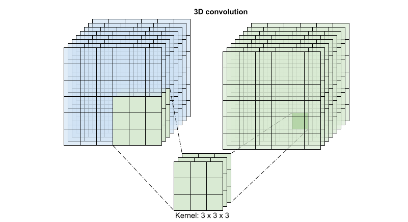
이 작업은 time * height * width * channels를 입력 받고 channels 출력을 생성합니다(입력 및 출력 채널의 수가 같다고 가정합니다. 따라서 커널 크기가 (3 x 3 x 3)인 3D 컨볼루션 레이어에는 27 * channels ** 2개 항목을 가진 가중치-행렬이 필요합니다). 참조 논문에서는 컨볼루션을 분해하는 것이 보다 효과적이고 효율적인 접근 방식임을 발견했습니다. 시간 및 공간 차원을 처리하기 위한 단일 3D 컨볼루션 대신 그들은 공간과 시간 차원을 별도로 처리하는 "(2+1 )D" 컨볼루션을 제안했습니다. 아래 그림은 (2 + 1)D 컨볼루션의 분해된 공간 및 시간 컨볼루션을 보여줍니다.

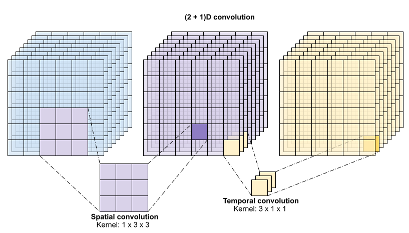
이 접근 방식의 주된 이점은 매개변수의 수를 줄이는 것입니다. (2 + 1)D 컨볼루션에서 공간 컨볼루션은 (1, width, height) 형상의 데이터를 받는 반면 시간 컨볼루션은 (time, 1, 1) 형상의 데이터를 받습니다. 예를 들어, 커널 크기가 (3 x 3 x 3)인 (2 + 1)D 컨볼루션에는 (9 * channels**2) + (3 * channels**2) 크기의 가중치 행렬이 필요합니다. 이는 많아야 전체 3D 컨볼루션의 절반 미만입니다. 이 튜토리얼에서는 resnet의 각 컨볼루션이 (2+1)D 컨볼루션으로 대체되는 (2 + 1)D ResNet18을 구현합니다.

# Define the dimensions of one frame in the set of frames created
HEIGHT = 224
WIDTH = 224

class Conv2Plus1D(keras.layers.Layer):
  def __init__(self, filters, kernel_size, padding):
    """
      A sequence of convolutional layers that first apply the convolution operation over the
      spatial dimensions, and then the temporal dimension. 
    """
    super().__init__()
    self.seq = keras.Sequential([  
        # Spatial decomposition
        layers.Conv3D(filters=filters,
                      kernel_size=(1, kernel_size[1], kernel_size[2]),
                      padding=padding),
        # Temporal decomposition
        layers.Conv3D(filters=filters, 
                      kernel_size=(kernel_size[0], 1, 1),
                      padding=padding)
        ])
  
  def call(self, x):
    return self.seq(x)

ResNet 모델은 잔차 블록 시퀀스로부터 만들어집니다. 잔차 블록에는 두 개의 분기가 있습니다. 주 분기는 계산을 수행하지만 그래디언트가 흐르기 어렵습니다. 전차 분기는 기본 계산을 우회하고 대부분 주 분기의 출력에 입력을 추가합니다. 그래디언트는 이 분기를 통해 쉽게 흐릅니다. 따라서 손실 함수에서 잔차 블록의 주 분기로 쉽게 이동할 수 있습니다. 그러면 그래디언트 소실 문제를 피할 수 있습니다.

다음 클래스를 사용하여 잔차 블록의 주 분기를 만듭니다. 표준 ResNet 구조와 달리 이는 layers.Conv2D 대신 사용자 정의 Conv2Plus1D 레이어를 사용합니다.

class ResidualMain(keras.layers.Layer):
  """
    Residual block of the model with convolution, layer normalization, and the
    activation function, ReLU.
  """
  def __init__(self, filters, kernel_size):
    super().__init__()
    self.seq = keras.Sequential([
        Conv2Plus1D(filters=filters,
                    kernel_size=kernel_size,
                    padding='same'),
        layers.LayerNormalization(),
        layers.ReLU(),
        Conv2Plus1D(filters=filters, 
                    kernel_size=kernel_size,
                    padding='same'),
        layers.LayerNormalization()
    ])
    
  def call(self, x):
    return self.seq(x)

잔차 분기를 주 분기에 추가하려면 크기가 같아야 합니다. 아래의 Project 레이어는 분기에서 채널 수가 변경되는 경우를 다룹니다. 특히, 밀집 연결된 레이어에 정규화가 뒤따르는 시퀀스가 추가됩니다.

class Project(keras.layers.Layer):
  """
    Project certain dimensions of the tensor as the data is passed through different 
    sized filters and downsampled. 
  """
  def __init__(self, units):
    super().__init__()
    self.seq = keras.Sequential([
        layers.Dense(units),
        layers.LayerNormalization()
    ])

  def call(self, x):
    return self.seq(x)

add_residual_block을 사용하여 모델 레이어 간에 건너뛰기 연결을 도입합니다.

def add_residual_block(input, filters, kernel_size):
  """
    Add residual blocks to the model. If the last dimensions of the input data
    and filter size does not match, project it such that last dimension matches.
  """
  out = ResidualMain(filters, 
                     kernel_size)(input)
  
  res = input
  # Using the Keras functional APIs, project the last dimension of the tensor to
  # match the new filter size
  if out.shape[-1] != input.shape[-1]:
    res = Project(out.shape[-1])(res)

  return layers.add([res, out])

데이터의 다운샘플링을 수행하려면 비디오 크기를 조정해야 합니다. 특히, 비디오 프레임을 다운샘플링하면 모델이 프레임의 특정 부분을 검사하여 특정 동작에 해당하는 패턴을 감지할 수 있습니다. 다운샘플링을 통해 중요하지 않은 정보를 버릴 수 있습니다. 또한 비디오 크기를 조정하면 차원 축소가 가능하므로 모델을 통한 처리 속도가 빨라집니다.

class ResizeVideo(keras.layers.Layer):
  def __init__(self, height, width):
    super().__init__()
    self.height = height
    self.width = width
    self.resizing_layer = layers.Resizing(self.height, self.width)

  def call(self, video):
    """
      Use the einops library to resize the tensor.  
      
      Args:
        video: Tensor representation of the video, in the form of a set of frames.
      
      Return:
        A downsampled size of the video according to the new height and width it should be resized to.
    """
    # b stands for batch size, t stands for time, h stands for height, 
    # w stands for width, and c stands for the number of channels.
    old_shape = einops.parse_shape(video, 'b t h w c')
    images = einops.rearrange(video, 'b t h w c -> (b t) h w c')
    images = self.resizing_layer(images)
    videos = einops.rearrange(
        images, '(b t) h w c -> b t h w c',
        t = old_shape['t'])
    return videos

Keras 함수형 API를 사용하여 잔차 네트워크를 구축합니다.

input_shape = (None, 10, HEIGHT, WIDTH, 3)
input = layers.Input(shape=(input_shape[1:]))
x = input

x = Conv2Plus1D(filters=16, kernel_size=(3, 7, 7), padding='same')(x)
x = layers.BatchNormalization()(x)
x = layers.ReLU()(x)
x = ResizeVideo(HEIGHT // 2, WIDTH // 2)(x)

# Block 1
x = add_residual_block(x, 16, (3, 3, 3))
x = ResizeVideo(HEIGHT // 4, WIDTH // 4)(x)

# Block 2
x = add_residual_block(x, 32, (3, 3, 3))
x = ResizeVideo(HEIGHT // 8, WIDTH // 8)(x)

# Block 3
x = add_residual_block(x, 64, (3, 3, 3))
x = ResizeVideo(HEIGHT // 16, WIDTH // 16)(x)

# Block 4
x = add_residual_block(x, 128, (3, 3, 3))

x = layers.GlobalAveragePooling3D()(x)
x = layers.Flatten()(x)
x = layers.Dense(10)(x)

model = keras.Model(input, x)

frames, label = next(iter(train_ds))
model.build(frames)

# Visualize the model
keras.utils.plot_model(model, expand_nested=True, dpi=60, show_shapes=True)

모델 훈련

이 튜토리얼에서는 tf.keras.optimizers.Adam 옵티마이저와 tf.keras.losses.SparseCategoricalCrossentropy 손실 함수를 선택합니다. 모든 단계에서 모델 성능의 정확도를 보려면 metrics 인수를 사용합니다.

model.compile(loss = keras.losses.SparseCategoricalCrossentropy(from_logits=True), 
              optimizer = keras.optimizers.Adam(learning_rate = 0.0001), 
              metrics = ['accuracy'])

Model.fit 메서드로 50 epoch 동안 모델을 훈련시킵니다.

참고: 이 예제 모델은 이 튜토리얼의 교육 시간을 합리적으로 유지하기 위해 더 적은 데이터 포인트(300개의 훈련 및 100개의 검증 예제)에 대해 훈련되었습니다. 또한 이 예제 모델은 훈련하는 데 1시간 이상 걸릴 수 있습니다.

history = model.fit(x = train_ds,
                    epochs = 50, 
                    validation_data = val_ds)

결과 시각화

훈련 및 검증 세트에 대한 손실 및 정확도 플롯을 생성합니다.

def plot_history(history):
  """
    Plotting training and validation learning curves.

    Args:
      history: model history with all the metric measures
  """
  fig, (ax1, ax2) = plt.subplots(2)

  fig.set_size_inches(18.5, 10.5)

  # Plot loss
  ax1.set_title('Loss')
  ax1.plot(history.history['loss'], label = 'train')
  ax1.plot(history.history['val_loss'], label = 'test')
  ax1.set_ylabel('Loss')
  
  # Determine upper bound of y-axis
  max_loss = max(history.history['loss'] + history.history['val_loss'])

  ax1.set_ylim([0, np.ceil(max_loss)])
  ax1.set_xlabel('Epoch')
  ax1.legend(['Train', 'Validation']) 

  # Plot accuracy
  ax2.set_title('Accuracy')
  ax2.plot(history.history['accuracy'],  label = 'train')
  ax2.plot(history.history['val_accuracy'], label = 'test')
  ax2.set_ylabel('Accuracy')
  ax2.set_ylim([0, 1])
  ax2.set_xlabel('Epoch')
  ax2.legend(['Train', 'Validation'])

  plt.show()

plot_history(history)

모델 평가하기

Keras Model.evaluate를 사용하여 테스트 데이터세트의 손실 및 정확도를 가져옵니다.

참고: 이 튜토리얼의 예제 모델은 훈련 시간을 합리적으로 유지하기 위해 UCF101 데이터세트의 일부만 사용합니다. 추가 하이퍼파라미터 조정이나 더 많은 훈련 데이터로 정확도와 손실을 개선할 수 있습니다.

model.evaluate(test_ds, return_dict=True)

모델 성능을 더 시각화하려면 혼동 행렬을 사용합니다. 혼동 행렬을 사용하면 정확도를 넘어 분류 모델의 성능을 평가할 수 있습니다. 이 다중 클래스 분류 문제에 대한 혼동 행렬을 작성하기 위해 테스트 세트의 실제 값과 예측 값을 가져옵니다.

def get_actual_predicted_labels(dataset): 
  """
    Create a list of actual ground truth values and the predictions from the model.

    Args:
      dataset: An iterable data structure, such as a TensorFlow Dataset, with features and labels.

    Return:
      Ground truth and predicted values for a particular dataset.
  """
  actual = [labels for _, labels in dataset.unbatch()]
  predicted = model.predict(dataset)

  actual = tf.stack(actual, axis=0)
  predicted = tf.concat(predicted, axis=0)
  predicted = tf.argmax(predicted, axis=1)

  return actual, predicted

def plot_confusion_matrix(actual, predicted, labels, ds_type):
  cm = tf.math.confusion_matrix(actual, predicted)
  ax = sns.heatmap(cm, annot=True, fmt='g')
  sns.set(rc={'figure.figsize':(12, 12)})
  sns.set(font_scale=1.4)
  ax.set_title('Confusion matrix of action recognition for ' + ds_type)
  ax.set_xlabel('Predicted Action')
  ax.set_ylabel('Actual Action')
  plt.xticks(rotation=90)
  plt.yticks(rotation=0)
  ax.xaxis.set_ticklabels(labels)
  ax.yaxis.set_ticklabels(labels)

fg = FrameGenerator(subset_paths['train'], n_frames, training=True)
labels = list(fg.class_ids_for_name.keys())

actual, predicted = get_actual_predicted_labels(train_ds)
plot_confusion_matrix(actual, predicted, labels, 'training')

actual, predicted = get_actual_predicted_labels(test_ds)
plot_confusion_matrix(actual, predicted, labels, 'test')

각 클래스의 정밀도와 호출 값은 혼동 행렬을 사용하여 계산할 수도 있습니다.

def calculate_classification_metrics(y_actual, y_pred, labels):
  """
    Calculate the precision and recall of a classification model using the ground truth and
    predicted values. 

    Args:
      y_actual: Ground truth labels.
      y_pred: Predicted labels.
      labels: List of classification labels.

    Return:
      Precision and recall measures.
  """
  cm = tf.math.confusion_matrix(y_actual, y_pred)
  tp = np.diag(cm) # Diagonal represents true positives
  precision = dict()
  recall = dict()
  for i in range(len(labels)):
    col = cm[:, i]
    fp = np.sum(col) - tp[i] # Sum of column minus true positive is false negative
    
    row = cm[i, :]
    fn = np.sum(row) - tp[i] # Sum of row minus true positive, is false negative
    
    precision[labels[i]] = tp[i] / (tp[i] + fp) # Precision 
    
    recall[labels[i]] = tp[i] / (tp[i] + fn) # Recall
  
  return precision, recall

precision, recall = calculate_classification_metrics(actual, predicted, labels) # Test dataset

precision

recall

다음 단계

TensorFlow에서 비디오 데이터 작업에 대해 자세히 알아보려면 다음 튜토리얼을 확인하세요.

• 비디오 데이터 로드

• 스트리밍 동작 인식을 위한 MoViNet

• MoViNet을 사용한 비디오 분류 전이 학습