GitHub Repository: tensorflow/docs-l10n
Path: blob/master/site/pt-br/tutorials/video/video_classification.ipynb
²⁵¹¹⁸ views

Kernel: Python 3

Copyright 2022 The TensorFlow Authors.

In [ ]:

#@title Licensed under the Apache License, Version 2.0 (the "License");
# you may not use this file except in compliance with the License.
# You may obtain a copy of the License at
#
# https://www.apache.org/licenses/LICENSE-2.0
#
# Unless required by applicable law or agreed to in writing, software
# distributed under the License is distributed on an "AS IS" BASIS,
# WITHOUT WARRANTIES OR CONDITIONS OF ANY KIND, either express or implied.
# See the License for the specific language governing permissions and
# limitations under the License.

Ver em TensorFlow.org

Executar no Google Colab

Ver fonte no GitHub

Baixar notebook

Classificação de vídeos com uma rede neural convolucional 3D

Este tutorial demonstra o treinamento de uma rede neural convolucional (CNN) 3D para classificação de vídeo usando o dataset de reconhecimento de ações UCF101. Uma CNN 3D usa um filtro tridimensional para realizar convoluções. O kernel é capaz de deslizar em três direções, enquanto que numa CNN 2D ele pode deslizar em duas dimensões. O modelo é baseado no trabalho publicado em A Closer Look at Spatiotemporal Convolutions for Action Recognition por D. Tran et al. (2017). Neste tutorial, você irá:

Construir um pipeline de entrada
Construir um modelo de rede neural convolucional 3D com conexões residuais usando a API funcional Keras
Treinar o modelo
Avaliar e testar o modelo

Este tutorial de classificação de vídeo é a segunda parte de uma série de tutoriais em vídeo do TensorFlow. Aqui estão os outros três tutoriais:

Carregando dados de vídeo: Este tutorial explica grande parte do código usado neste documento.
MoViNet para o reconhecimento de ações de streaming: conheça os modelos MoViNet disponíveis no TF Hub.
Aprendizado por transferência para a classificação de vídeos com MoViNet: este tutorial explica como usar um modelo de classificação de vídeos pré-treinado em um dataset diferente com o dataset UCF-101.

Configuração

Comece instalando e importando algumas bibliotecas necessárias, incluindo: remotezip para inspecionar o conteúdo de um arquivo ZIP, tqdm para usar uma barra de progresso, OpenCV para processar arquivos de vídeo, einops para realizar operações de tensor mais complexas e tensorflow_docs para incorporar dados em um notebook Jupyter.

Observação: use o TensorFlow 2.10 para executar este tutorial. Versões acima do TensorFlow 2.10 podem não ser executadas com sucesso.

In [ ]:

!pip install remotezip tqdm opencv-python einops 
# Install TensorFlow 2.10
!pip install tensorflow==2.10.0

In [ ]:

import tqdm
import random
import pathlib
import itertools
import collections

import cv2
import einops
import numpy as np
import remotezip as rz
import seaborn as sns
import matplotlib.pyplot as plt

import tensorflow as tf
import keras
from keras import layers

Carregamento e pré-processamento dos dados de vídeo

A célula oculta abaixo define funções auxiliares para baixar uma fatia de dados do dataset UCF-101 e carregá-los num tf.data.Dataset. Você pode aprender mais sobre os passos específicos de pré-processamento no tutorial Carregando dados de vídeo, que apresenta instruções detalhadas sobre esse código.

A classe FrameGenerator no final do bloco oculto é o utilitário mais importante que temos aqui, pois cria um objeto iterável que pode alimentar dados no pipeline de dados do TensorFlow. Especificamente, essa classe contém um gerador Python que carrega os quadros do vídeo juntamente com seu rótulo codificado. A função geradora (__call__) gera a array de quadros produzida por frames_from_video_file e um vetor com codificação one-hot do rótulo associado ao conjunto de quadros.

In [ ]:

#@title

def list_files_per_class(zip_url):
  """
    List the files in each class of the dataset given the zip URL.

    Args:
      zip_url: URL from which the files can be unzipped. 

    Return:
      files: List of files in each of the classes.
  """
  files = []
  with rz.RemoteZip(URL) as zip:
    for zip_info in zip.infolist():
      files.append(zip_info.filename)
  return files

def get_class(fname):
  """
    Retrieve the name of the class given a filename.

    Args:
      fname: Name of the file in the UCF101 dataset.

    Return:
      Class that the file belongs to.
  """
  return fname.split('_')[-3]

def get_files_per_class(files):
  """
    Retrieve the files that belong to each class. 

    Args:
      files: List of files in the dataset.

    Return:
      Dictionary of class names (key) and files (values).
  """
  files_for_class = collections.defaultdict(list)
  for fname in files:
    class_name = get_class(fname)
    files_for_class[class_name].append(fname)
  return files_for_class

def download_from_zip(zip_url, to_dir, file_names):
  """
    Download the contents of the zip file from the zip URL.

    Args:
      zip_url: Zip URL containing data.
      to_dir: Directory to download data to.
      file_names: Names of files to download.
  """
  with rz.RemoteZip(zip_url) as zip:
    for fn in tqdm.tqdm(file_names):
      class_name = get_class(fn)
      zip.extract(fn, str(to_dir / class_name))
      unzipped_file = to_dir / class_name / fn

      fn = pathlib.Path(fn).parts[-1]
      output_file = to_dir / class_name / fn
      unzipped_file.rename(output_file,)

def split_class_lists(files_for_class, count):
  """
    Returns the list of files belonging to a subset of data as well as the remainder of
    files that need to be downloaded.
    
    Args:
      files_for_class: Files belonging to a particular class of data.
      count: Number of files to download.

    Return:
      split_files: Files belonging to the subset of data.
      remainder: Dictionary of the remainder of files that need to be downloaded.
  """
  split_files = []
  remainder = {}
  for cls in files_for_class:
    split_files.extend(files_for_class[cls][:count])
    remainder[cls] = files_for_class[cls][count:]
  return split_files, remainder

def download_ufc_101_subset(zip_url, num_classes, splits, download_dir):
  """
    Download a subset of the UFC101 dataset and split them into various parts, such as
    training, validation, and test. 

    Args:
      zip_url: Zip URL containing data.
      num_classes: Number of labels.
      splits: Dictionary specifying the training, validation, test, etc. (key) division of data 
              (value is number of files per split).
      download_dir: Directory to download data to.

    Return:
      dir: Posix path of the resulting directories containing the splits of data.
  """
  files = list_files_per_class(zip_url)
  for f in files:
    tokens = f.split('/')
    if len(tokens) <= 2:
      files.remove(f) # Remove that item from the list if it does not have a filename
  
  files_for_class = get_files_per_class(files)

  classes = list(files_for_class.keys())[:num_classes]

  for cls in classes:
    new_files_for_class = files_for_class[cls]
    random.shuffle(new_files_for_class)
    files_for_class[cls] = new_files_for_class
    
  # Only use the number of classes you want in the dictionary
  files_for_class = {x: files_for_class[x] for x in list(files_for_class)[:num_classes]}

  dirs = {}
  for split_name, split_count in splits.items():
    print(split_name, ":")
    split_dir = download_dir / split_name
    split_files, files_for_class = split_class_lists(files_for_class, split_count)
    download_from_zip(zip_url, split_dir, split_files)
    dirs[split_name] = split_dir

  return dirs

def format_frames(frame, output_size):
  """
    Pad and resize an image from a video.
    
    Args:
      frame: Image that needs to resized and padded. 
      output_size: Pixel size of the output frame image.

    Return:
      Formatted frame with padding of specified output size.
  """
  frame = tf.image.convert_image_dtype(frame, tf.float32)
  frame = tf.image.resize_with_pad(frame, *output_size)
  return frame

def frames_from_video_file(video_path, n_frames, output_size = (224,224), frame_step = 15):
  """
    Creates frames from each video file present for each category.

    Args:
      video_path: File path to the video.
      n_frames: Number of frames to be created per video file.
      output_size: Pixel size of the output frame image.

    Return:
      An NumPy array of frames in the shape of (n_frames, height, width, channels).
  """
  # Read each video frame by frame
  result = []
  src = cv2.VideoCapture(str(video_path))  

  video_length = src.get(cv2.CAP_PROP_FRAME_COUNT)

  need_length = 1 + (n_frames - 1) * frame_step

  if need_length > video_length:
    start = 0
  else:
    max_start = video_length - need_length
    start = random.randint(0, max_start + 1)

  src.set(cv2.CAP_PROP_POS_FRAMES, start)
  # ret is a boolean indicating whether read was successful, frame is the image itself
  ret, frame = src.read()
  result.append(format_frames(frame, output_size))

  for _ in range(n_frames - 1):
    for _ in range(frame_step):
      ret, frame = src.read()
    if ret:
      frame = format_frames(frame, output_size)
      result.append(frame)
    else:
      result.append(np.zeros_like(result[0]))
  src.release()
  result = np.array(result)[..., [2, 1, 0]]

  return result

class FrameGenerator:
  def __init__(self, path, n_frames, training = False):
    """ Returns a set of frames with their associated label. 

      Args:
        path: Video file paths.
        n_frames: Number of frames. 
        training: Boolean to determine if training dataset is being created.
    """
    self.path = path
    self.n_frames = n_frames
    self.training = training
    self.class_names = sorted(set(p.name for p in self.path.iterdir() if p.is_dir()))
    self.class_ids_for_name = dict((name, idx) for idx, name in enumerate(self.class_names))

  def get_files_and_class_names(self):
    video_paths = list(self.path.glob('*/*.avi'))
    classes = [p.parent.name for p in video_paths] 
    return video_paths, classes

  def __call__(self):
    video_paths, classes = self.get_files_and_class_names()

    pairs = list(zip(video_paths, classes))

    if self.training:
      random.shuffle(pairs)

    for path, name in pairs:
      video_frames = frames_from_video_file(path, self.n_frames) 
      label = self.class_ids_for_name[name] # Encode labels
      yield video_frames, label

In [ ]:

URL = 'https://storage.googleapis.com/thumos14_files/UCF101_videos.zip'
download_dir = pathlib.Path('./UCF101_subset/')
subset_paths = download_ufc_101_subset(URL, 
                        num_classes = 10, 
                        splits = {"train": 30, "val": 10, "test": 10},
                        download_dir = download_dir)

Crie os datasets de treinamento, validação e teste (train_ds , val_ds e test_ds).

In [ ]:

n_frames = 10
batch_size = 8

output_signature = (tf.TensorSpec(shape = (None, None, None, 3), dtype = tf.float32),
                    tf.TensorSpec(shape = (), dtype = tf.int16))

train_ds = tf.data.Dataset.from_generator(FrameGenerator(subset_paths['train'], n_frames, training=True),
                                          output_signature = output_signature)


# Batch the data
train_ds = train_ds.batch(batch_size)

val_ds = tf.data.Dataset.from_generator(FrameGenerator(subset_paths['val'], n_frames),
                                        output_signature = output_signature)
val_ds = val_ds.batch(batch_size)

test_ds = tf.data.Dataset.from_generator(FrameGenerator(subset_paths['test'], n_frames),
                                         output_signature = output_signature)

test_ds = test_ds.batch(batch_size)

Criação do modelo

O seguinte modelo de rede neural convolucional 3D é baseado no artigo A Closer Look at Spatiotemporal Convolutions for Action Recognition de D. Tran et al. (2017). O artigo compara várias versões de ResNets 3D. Em vez de operar em uma única imagem com dimensões (height, width), como os ResNets padrão, estes operam no volume do vídeo (time, height, width). A abordagem mais óbvia para este problema seria substituir cada convolução 2D (layers.Conv2D) por uma convolução 3D (layers.Conv3D).

Este tutorial usa uma convolução (2 + 1)D com conexões residuais. A convolução (2 + 1)D permite a decomposição das dimensões espacial e temporal, criando assim dois passos distintos. Uma vantagem desta abordagem é que a fatoração das convoluções em dimensões espaciais e temporais economiza parâmetros.

Para cada local de saída, uma convolução 3D combina todos os vetores de um patch 3D do volume para criar um vetor no volume de saída.

3D convolutions

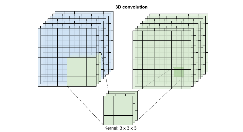
Esta operação leva time * height * width * channels e produz saídas channels (assumindo que o número de canais de entrada e saída são iguais. Portanto, uma camada de convolução 3D com um tamanho de kernel de (3 x 3 x 3) precisaria de uma matriz de pesos com 27 * channels ** 2 entradas. O artigo de referência descobriu que uma abordagem mais eficaz e eficiente era fatorar a convolução. Em vez de uma única convolução 3D para processar as dimensões de tempo e espaço, eles propuseram uma convolução "(2+1 )D" que processa as dimensões de espaço e tempo separadamente. A figura abaixo mostra as convoluções espaciais e temporais fatoradas de uma convolução (2 + 1)D.

(2+1)D convolutions

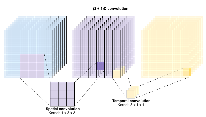
A principal vantagem desta abordagem é que ela reduz o número de parâmetros. Na convolução (2 + 1)D, a convolução espacial recebe dados no formato (1, width, height), enquanto a convolução temporal recebe dados no formato (time, 1, 1). Por exemplo, uma convolução (2 + 1)D com tamanho de kernel (3 x 3 x 3) precisaria de matrizes de peso de tamanho (9 * channels**2) + (3 * channels**2), menos da metade da convolução 3D completa. Este tutorial implementa (2 + 1)D ResNet18, onde cada convolução na resnet é substituída por uma convolução (2+1)D.

In [ ]:

# Define the dimensions of one frame in the set of frames created
HEIGHT = 224
WIDTH = 224

In [ ]:

class Conv2Plus1D(keras.layers.Layer):
  def __init__(self, filters, kernel_size, padding):
    """
      A sequence of convolutional layers that first apply the convolution operation over the
      spatial dimensions, and then the temporal dimension. 
    """
    super().__init__()
    self.seq = keras.Sequential([  
        # Spatial decomposition
        layers.Conv3D(filters=filters,
                      kernel_size=(1, kernel_size[1], kernel_size[2]),
                      padding=padding),
        # Temporal decomposition
        layers.Conv3D(filters=filters, 
                      kernel_size=(kernel_size[0], 1, 1),
                      padding=padding)
        ])
  
  def call(self, x):
    return self.seq(x)

Um modelo ResNet é feito a partir de uma sequência de blocos residuais. Um bloco residual possui duas ramificações. O ramo principal realiza o cálculo, mas dificulta o fluxo dos gradientes. A ramificação residual ignora o cálculo principal e geralmente apenas adiciona a entrada à saída da ramificação principal. Os gradientes fluem facilmente através deste ramo. Portanto, um caminho fácil da função de perda para qualquer ramo principal do bloco residual estará presente. Isto evita o problema do sumiço do gradiente.

Crie a ramificação principal do bloco residual com a seguinte classe. Em contraste com a estrutura ResNet padrão, esta usa a camada Conv2Plus1D personalizada em vez de layers.Conv2D.

In [ ]:

class ResidualMain(keras.layers.Layer):
  """
    Residual block of the model with convolution, layer normalization, and the
    activation function, ReLU.
  """
  def __init__(self, filters, kernel_size):
    super().__init__()
    self.seq = keras.Sequential([
        Conv2Plus1D(filters=filters,
                    kernel_size=kernel_size,
                    padding='same'),
        layers.LayerNormalization(),
        layers.ReLU(),
        Conv2Plus1D(filters=filters, 
                    kernel_size=kernel_size,
                    padding='same'),
        layers.LayerNormalization()
    ])
    
  def call(self, x):
    return self.seq(x)

Para adicionar o ramo residual ao ramo principal ele precisa ter o mesmo tamanho. A camada Project abaixo trata dos casos em que o número de canais é alterado na ramificação. No caso em particular, é adicionada uma sequência de camadas densamente conectadas seguida de normalização.

In [ ]:

class Project(keras.layers.Layer):
  """
    Project certain dimensions of the tensor as the data is passed through different 
    sized filters and downsampled. 
  """
  def __init__(self, units):
    super().__init__()
    self.seq = keras.Sequential([
        layers.Dense(units),
        layers.LayerNormalization()
    ])

  def call(self, x):
    return self.seq(x)

Use add_residual_block para introduzir uma conexão de salto entre as camadas do modelo.

In [ ]:

def add_residual_block(input, filters, kernel_size):
  """
    Add residual blocks to the model. If the last dimensions of the input data
    and filter size does not match, project it such that last dimension matches.
  """
  out = ResidualMain(filters, 
                     kernel_size)(input)
  
  res = input
  # Using the Keras functional APIs, project the last dimension of the tensor to
  # match the new filter size
  if out.shape[-1] != input.shape[-1]:
    res = Project(out.shape[-1])(res)

  return layers.add([res, out])

O redimensionamento do vídeo é necessário para realizar a redução da resolução dos dados. Em particular, a redução da resolução dos quadros de vídeo permite que o modelo examine partes específicas dos quadros para detectar padrões que podem ser específicos de uma determinada ação. Através da redução da resolução, informações não essenciais podem ser descartadas. Além disso, o redimensionamento do vídeo permitirá a redução da dimensionalidade e garantirá, portanto, um processamento mais rápido através do modelo.

In [ ]:

class ResizeVideo(keras.layers.Layer):
  def __init__(self, height, width):
    super().__init__()
    self.height = height
    self.width = width
    self.resizing_layer = layers.Resizing(self.height, self.width)

  def call(self, video):
    """
      Use the einops library to resize the tensor.  
      
      Args:
        video: Tensor representation of the video, in the form of a set of frames.
      
      Return:
        A downsampled size of the video according to the new height and width it should be resized to.
    """
    # b stands for batch size, t stands for time, h stands for height, 
    # w stands for width, and c stands for the number of channels.
    old_shape = einops.parse_shape(video, 'b t h w c')
    images = einops.rearrange(video, 'b t h w c -> (b t) h w c')
    images = self.resizing_layer(images)
    videos = einops.rearrange(
        images, '(b t) h w c -> b t h w c',
        t = old_shape['t'])
    return videos

Use a API funcional Keras para construir a rede residual.

In [ ]:

input_shape = (None, 10, HEIGHT, WIDTH, 3)
input = layers.Input(shape=(input_shape[1:]))
x = input

x = Conv2Plus1D(filters=16, kernel_size=(3, 7, 7), padding='same')(x)
x = layers.BatchNormalization()(x)
x = layers.ReLU()(x)
x = ResizeVideo(HEIGHT // 2, WIDTH // 2)(x)

# Block 1
x = add_residual_block(x, 16, (3, 3, 3))
x = ResizeVideo(HEIGHT // 4, WIDTH // 4)(x)

# Block 2
x = add_residual_block(x, 32, (3, 3, 3))
x = ResizeVideo(HEIGHT // 8, WIDTH // 8)(x)

# Block 3
x = add_residual_block(x, 64, (3, 3, 3))
x = ResizeVideo(HEIGHT // 16, WIDTH // 16)(x)

# Block 4
x = add_residual_block(x, 128, (3, 3, 3))

x = layers.GlobalAveragePooling3D()(x)
x = layers.Flatten()(x)
x = layers.Dense(10)(x)

model = keras.Model(input, x)

In [ ]:

frames, label = next(iter(train_ds))
model.build(frames)

In [ ]:

# Visualize the model
keras.utils.plot_model(model, expand_nested=True, dpi=60, show_shapes=True)

Treinamento do modelo

Neste tutorial, escolha o otimizador tf.keras.optimizers.Adam e a função de perda tf.keras.losses.SparseCategoricalCrossentropy. Use o argumento metrics para ver a exatidão do desempenho do modelo a cada passo.

In [ ]:

model.compile(loss = keras.losses.SparseCategoricalCrossentropy(from_logits=True), 
              optimizer = keras.optimizers.Adam(learning_rate = 0.0001), 
              metrics = ['accuracy'])

Treine o modelo com 50 épocas usando o método Model.fit do Keras:

Observação: Este modelo de exemplo é treinado em menos pontos de dados (300 exemplos de treinamento e 100 exemplos de validação) para manter o tempo de treinamento razoável para este tutorial. Além disso, este modelo de exemplo pode levar mais de uma hora para ser treinado.

In [ ]:

history = model.fit(x = train_ds,
                    epochs = 50, 
                    validation_data = val_ds)

Visualize os resultados

Crie gráficos da perda e da exatidão para os conjuntos de treinamento e avaliação:

In [ ]:

def plot_history(history):
  """
    Plotting training and validation learning curves.

    Args:
      history: model history with all the metric measures
  """
  fig, (ax1, ax2) = plt.subplots(2)

  fig.set_size_inches(18.5, 10.5)

  # Plot loss
  ax1.set_title('Loss')
  ax1.plot(history.history['loss'], label = 'train')
  ax1.plot(history.history['val_loss'], label = 'test')
  ax1.set_ylabel('Loss')
  
  # Determine upper bound of y-axis
  max_loss = max(history.history['loss'] + history.history['val_loss'])

  ax1.set_ylim([0, np.ceil(max_loss)])
  ax1.set_xlabel('Epoch')
  ax1.legend(['Train', 'Validation']) 

  # Plot accuracy
  ax2.set_title('Accuracy')
  ax2.plot(history.history['accuracy'],  label = 'train')
  ax2.plot(history.history['val_accuracy'], label = 'test')
  ax2.set_ylabel('Accuracy')
  ax2.set_ylim([0, 1])
  ax2.set_xlabel('Epoch')
  ax2.legend(['Train', 'Validation'])

  plt.show()

plot_history(history)

Avaliação do modelo

Use Model.evaluate do Keras para obter a perda e a precisão do dataset de dados de teste.

Observação: o modelo de exemplo neste tutorial usa um subconjunto do dataset UCF101 para manter o tempo de treinamento razoável. A precisão e a perda podem ser melhoradas com mais ajustes de hiperparâmetros ou mais dados de treinamento.

In [ ]:

model.evaluate(test_ds, return_dict=True)

Para avaliar o desempenho do modelo com mais detalhes, use uma matriz de confusão, que permite avaliar o desempenho do modelo de classificação além da exatidão. Para criar a matriz de confusão para este problema de classificação multiclasse, obtenha os valores reais do dataset de teste e os valores previstos.

In [ ]:

def get_actual_predicted_labels(dataset): 
  """
    Create a list of actual ground truth values and the predictions from the model.

    Args:
      dataset: An iterable data structure, such as a TensorFlow Dataset, with features and labels.

    Return:
      Ground truth and predicted values for a particular dataset.
  """
  actual = [labels for _, labels in dataset.unbatch()]
  predicted = model.predict(dataset)

  actual = tf.stack(actual, axis=0)
  predicted = tf.concat(predicted, axis=0)
  predicted = tf.argmax(predicted, axis=1)

  return actual, predicted

In [ ]:

def plot_confusion_matrix(actual, predicted, labels, ds_type):
  cm = tf.math.confusion_matrix(actual, predicted)
  ax = sns.heatmap(cm, annot=True, fmt='g')
  sns.set(rc={'figure.figsize':(12, 12)})
  sns.set(font_scale=1.4)
  ax.set_title('Confusion matrix of action recognition for ' + ds_type)
  ax.set_xlabel('Predicted Action')
  ax.set_ylabel('Actual Action')
  plt.xticks(rotation=90)
  plt.yticks(rotation=0)
  ax.xaxis.set_ticklabels(labels)
  ax.yaxis.set_ticklabels(labels)

In [ ]:

fg = FrameGenerator(subset_paths['train'], n_frames, training=True)
labels = list(fg.class_ids_for_name.keys())

In [ ]:

actual, predicted = get_actual_predicted_labels(train_ds)
plot_confusion_matrix(actual, predicted, labels, 'training')

In [ ]:

actual, predicted = get_actual_predicted_labels(test_ds)
plot_confusion_matrix(actual, predicted, labels, 'test')

Os valores de precisão e recuperação para cada classe também podem ser calculados usando uma matriz de confusão.

In [ ]:

def calculate_classification_metrics(y_actual, y_pred, labels):
  """
    Calculate the precision and recall of a classification model using the ground truth and
    predicted values. 

    Args:
      y_actual: Ground truth labels.
      y_pred: Predicted labels.
      labels: List of classification labels.

    Return:
      Precision and recall measures.
  """
  cm = tf.math.confusion_matrix(y_actual, y_pred)
  tp = np.diag(cm) # Diagonal represents true positives
  precision = dict()
  recall = dict()
  for i in range(len(labels)):
    col = cm[:, i]
    fp = np.sum(col) - tp[i] # Sum of column minus true positive is false negative
    
    row = cm[i, :]
    fn = np.sum(row) - tp[i] # Sum of row minus true positive, is false negative
    
    precision[labels[i]] = tp[i] / (tp[i] + fp) # Precision 
    
    recall[labels[i]] = tp[i] / (tp[i] + fn) # Recall
  
  return precision, recall

In [ ]:

precision, recall = calculate_classification_metrics(actual, predicted, labels) # Test dataset

In [ ]:

precision

In [ ]:

recall

Próximos passos

Para saber mais sobre como trabalhar com dados de vídeo no TensorFlow, confira os seguintes tutoriais: