Book a Demo!
CoCalc Logo Icon
StoreFeaturesDocsShareSupportNewsAboutPoliciesSign UpSign In
Download
45 views
unlisted
ubuntu1804

Tableau and toggle dynamics

Computation and visualization

Jessica Striker

If you're already using the computer to discover things, why not also use it to explain things!

Tableau Dynamics

A tableau is numbers in boxes with rules.

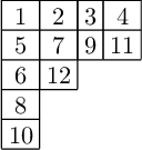
A standard Young tableaux is the numbers 1, 2, 3, ... in a partition shape of boxes, increasing along rows and columns, with each number used exactly once.

syt = StandardTableaux(12).random_element() show(syt)

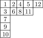
Now act on the tableau with promotion.

sytpro = syt.promotion_inverse() show(sytpro)

What just happened?

Let's write some code to help us visualize it.

def list_of_bender_knuth(tab): starting = deepcopy(tab) output = [tab] for i in range(len(tab.cells())-1): tab = tab.bender_knuth_involution(i+1) output.append(tab) return output def list_of_bender_knuth_plots(tab): output = [] lobk = list_of_bender_knuth(tab) m = len(lobk) for i in range(m-1): output.append(plot_highlight(lobk[i],[i+1,i+2])) output.append(plot_highlight(lobk[i+1],[i+1,i+2])) output.append(plot_highlight(lobk[m-1],[m-1,m])) return output def plot_highlight(tab,list_of_numbers_to_highlight): from sage.plot.polygon import polygon from sage.plot.line import line from sage.plot.text import text p = tab.shape() G = line([(0,0),(p[0],0)], axes=False, figsize=4.5) for i in range(len(p)): G += line([(0,-i-1), (p[i],-i-1)]) r = p.conjugate() G += line([(0,0),(0,-r[0])]) for i in range(len(r)): G += line([(i+1,0),(i+1,-r[i])]) for i in list_of_numbers_to_highlight: icells = tab.cells_containing(i) for c in icells: G += polygon([(c[1],-c[0]), (c[1]+1,-c[0]), (c[1]+1,-c[0]-1), (c[1],-c[0]-1)], rgbcolor=(1,0,1)) for c in tab.cells(): G += text(str(tab.entry(c)), (c[1]+0.5,-c[0]-0.5), fontsize = 'x-large') return G

Use the function 'animate' to see the visualizations compactly.

show ( animate(list_of_bender_knuth_plots(syt)), delay = 70 )

How did we write the code?

Look for code to modify.

syt.plot??

Generalize the tableaux.

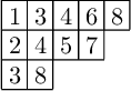
An increasing tableau is numbers in a partition shape of boxes, increasing in rows and columns.

(No rule about using numbers exactly once)
inct = IncreasingTableau([[1,2,4,5,7],[3,4,6,8],[4,5]]) show(inct)

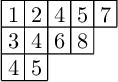
Act on an increasing tableau by K-Promotion.

inctpro = inct.K_promotion() show(inctpro)

Again, what just happened?

Let's write some code to help us visualize it.

def list_of_K_bender_knuth(tab,n): starting = deepcopy(tab) output = [tab] for i in range(n-1): tab = tab.K_bender_knuth(i+1) output.append(tab) return output def list_of_K_bender_knuth_plots(tab,n): output = [] lobk = list_of_K_bender_knuth(tab,n) m = len(lobk) for i in range(m-1): output.append(plot_highlight(lobk[i],[i+1,i+2])) output.append(plot_highlight(lobk[i+1],[i+1,i+2])) output.append(plot_highlight(lobk[m-1],[m-1,m])) return output
show ( animate(list_of_K_bender_knuth_plots(inct,8)), delay = 70 )

Toggle Dynamics

(The Hasse diagram of) a poset is numbers (elements) with arrows (covering relations) that are directed weakly upward.

Let's make a random poset.

P = Posets(7).random_element() plot(P)

An order ideal is a subset of poset elements that is closed downward.

Let's make a random order ideal.

oi = P.random_order_ideal() P.order_ideal_plot(oi)

Let's use different colors.

(This should be an option. Who wrote this code anyway?)
P.order_ideal_plot??
File: /ext/sage/sage-8.9_1804/local/lib/python2.7/site-packages/sage/combinat/posets/posets.py Source: def order_ideal_plot(self, elements): r""" Return a plot of the order ideal generated by the elements of an iterable ``elements``. `I` is an order ideal if, for any `x` in `I` and `y` such that `y \le x`, then `y` is in `I`. This is also called lower set or downset. EXAMPLES:: sage: P = Poset((divisors(1000), attrcall("divides"))) sage: P.order_ideal_plot([20, 25]) Graphics object consisting of 41 graphics primitives TESTS:: sage: P = Poset() # Test empty poset sage: P.order_ideal_plot([]) Graphics object consisting of 0 graphics primitives sage: C = posets.ChainPoset(5) sage: C.order_ideal_plot([]) Graphics object consisting of 10 graphics primitives """ order_ideal = self.order_ideal(elements) order_filer = self.order_filter(self.order_ideal_complement_generators(order_ideal)) order_ideal_color_dictionary = {} order_ideal_color_dictionary['green'] = order_ideal order_ideal_color_dictionary['red']= order_filer return self.plot(element_colors = order_ideal_color_dictionary)
def order_ideal_plot_colors(myposet, elements): order_ideal = myposet.order_ideal(elements) order_filer = myposet.order_filter(myposet.order_ideal_complement_generators(order_ideal)) order_ideal_color_dictionary = {} order_ideal_color_dictionary['blue'] = order_ideal order_ideal_color_dictionary['red']= order_filer return myposet.plot(label_elements = False, element_colors = order_ideal_color_dictionary)
order_ideal_plot_colors(P,oi)

Act on an order ideal by rowmotion.

rowoi = P.rowmotion(oi)

Should try to make our functions a little less persnickety...

The rowmotion function should be able to accept a list as input and then change it to a set.

rowoi = P.rowmotion(set(oi)) order_ideal_plot_colors(P,rowoi)

For a third time, what just happened?

Code and animations to the rescue!

#Colors the rowmotion generators yellow - only works since yellow is the last color to be colored (alphabetically last) def order_ideal_plot_colors_antichain(myposet, elements): order_ideal = myposet.order_ideal(elements) complement_gens = myposet.order_ideal_complement_generators(elements) order_filer = myposet.order_filter(myposet.order_ideal_complement_generators(order_ideal)) order_ideal_color_dictionary = {} order_ideal_color_dictionary['blue'] = order_ideal order_ideal_color_dictionary['yellow'] = complement_gens order_ideal_color_dictionary['red']= order_filer return myposet.plot(label_elements = False, element_colors = order_ideal_color_dictionary) #Rowmotion by convex closure def list_of_row_order_ideal_plots(myposet, elements): output = [] for orderideal in myposet.rowmotion_orbit_iter(elements): output.append(order_ideal_plot_colors(myposet, orderideal)) output.append(order_ideal_plot_colors_antichain(myposet, orderideal)) return output
show ( animate (list_of_row_order_ideal_plots(P,set(oi) )), delay = 100 )

Make a list of the elements of your poset, then a list of the covering relations between poset element.

Here are some of my favorite posets
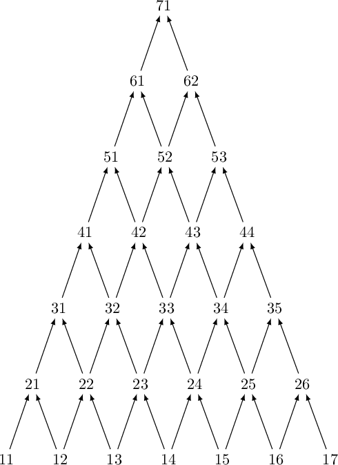
The triangle

elemP7 = [11, 12, 13, 14, 15, 16, 17, 21, 22, 23, 24, 25, 26, 31, 32, 33, 34, 35, 41, 42, 43, 44, 51, 52, 53, 61, 62, 71] relP7 = [[11,21],[12, 21],[12, 22],[13, 22],[13, 23],[14, 23],[14, 24],[15,24],[15,25],[16,25],[16,26],[17,26],[21,31],[22,31],[22,32],[23,32],[23,33],[24,33],[24,34],[25,34],[25,35],[26,35],[31,41],[32,41],[32,42],[33,42],[33,43],[34,43],[34,44],[35,44],[41,51],[42,51],[42,52],[43,52],[43,53],[44,53],[51,61],[52,61],[52,62],[52,62],[53,62],[61,71],[62,71]] P7 = Poset((elemP7,relP7))
plot(P7)

Some other ways to plot posets

The pretty way

show(P7)

For putting in your paper

latex(P7)
\begin{tikzpicture}[>=latex,line join=bevel,] %% \node (node_26) at (128.5bp,251.5bp) [draw,draw=none] {$62$}; \node (node_27) at (110.5bp,300.5bp) [draw,draw=none] {$71$}; \node (node_24) at (146.5bp,202.5bp) [draw,draw=none] {$53$}; \node (node_25) at (93.5bp,251.5bp) [draw,draw=none] {$61$}; \node (node_22) at (76.5bp,202.5bp) [draw,draw=none] {$51$}; \node (node_23) at (111.5bp,202.5bp) [draw,draw=none] {$52$}; \node (node_20) at (129.5bp,153.5bp) [draw,draw=none] {$43$}; \node (node_21) at (164.5bp,153.5bp) [draw,draw=none] {$44$}; \node (node_9) at (95.5bp,55.5bp) [draw,draw=none] {$23$}; \node (node_8) at (60.5bp,55.5bp) [draw,draw=none] {$22$}; \node (node_7) at (25.5bp,55.5bp) [draw,draw=none] {$21$}; \node (node_6) at (218.5bp,6.5bp) [draw,draw=none] {$17$}; \node (node_5) at (183.5bp,6.5bp) [draw,draw=none] {$16$}; \node (node_4) at (148.5bp,6.5bp) [draw,draw=none] {$15$}; \node (node_3) at (113.5bp,6.5bp) [draw,draw=none] {$14$}; \node (node_2) at (78.5bp,6.5bp) [draw,draw=none] {$13$}; \node (node_1) at (43.5bp,6.5bp) [draw,draw=none] {$12$}; \node (node_0) at (8.5bp,6.5bp) [draw,draw=none] {$11$}; \node (node_19) at (94.5bp,153.5bp) [draw,draw=none] {$42$}; \node (node_18) at (59.5bp,153.5bp) [draw,draw=none] {$41$}; \node (node_17) at (182.5bp,104.5bp) [draw,draw=none] {$35$}; \node (node_16) at (147.5bp,104.5bp) [draw,draw=none] {$34$}; \node (node_15) at (112.5bp,104.5bp) [draw,draw=none] {$33$}; \node (node_14) at (77.5bp,104.5bp) [draw,draw=none] {$32$}; \node (node_13) at (42.5bp,104.5bp) [draw,draw=none] {$31$}; \node (node_12) at (200.5bp,55.5bp) [draw,draw=none] {$26$}; \node (node_11) at (165.5bp,55.5bp) [draw,draw=none] {$25$}; \node (node_10) at (130.5bp,55.5bp) [draw,draw=none] {$24$}; \draw [black,->] (node_18) ..controls (64.173bp,166.97bp) and (67.775bp,177.35bp) .. (node_22); \draw [black,->] (node_6) ..controls (213.55bp,19.969bp) and (209.74bp,30.353bp) .. (node_12); \draw [black,->] (node_3) ..controls (118.17bp,19.969bp) and (121.78bp,30.353bp) .. (node_10); \draw [black,->] (node_23) ..controls (116.17bp,215.97bp) and (119.78bp,226.35bp) .. (node_26); \draw [black,->] (node_7) ..controls (30.173bp,68.969bp) and (33.775bp,79.353bp) .. (node_13); \draw [black,->] (node_16) ..controls (142.55bp,117.97bp) and (138.74bp,128.35bp) .. (node_20); \draw [black,->] (node_9) ..controls (100.17bp,68.969bp) and (103.78bp,79.353bp) .. (node_15); \draw [black,->] (node_10) ..controls (125.55bp,68.969bp) and (121.74bp,79.353bp) .. (node_15); \draw [black,->] (node_5) ..controls (178.55bp,19.969bp) and (174.74bp,30.353bp) .. (node_11); \draw [black,->] (node_0) ..controls (13.173bp,19.969bp) and (16.775bp,30.353bp) .. (node_7); \draw [black,->] (node_12) ..controls (195.55bp,68.969bp) and (191.74bp,79.353bp) .. (node_17); \draw [black,->] (node_4) ..controls (143.55bp,19.969bp) and (139.74bp,30.353bp) .. (node_10); \draw [black,->] (node_15) ..controls (117.17bp,117.97bp) and (120.78bp,128.35bp) .. (node_20); \draw [black,->] (node_26) ..controls (123.55bp,264.97bp) and (119.74bp,275.35bp) .. (node_27); \draw [black,->] (node_9) ..controls (90.552bp,68.969bp) and (86.738bp,79.353bp) .. (node_14); \draw [black,->] (node_3) ..controls (108.55bp,19.969bp) and (104.74bp,30.353bp) .. (node_9); \draw [black,->] (node_24) ..controls (141.55bp,215.97bp) and (137.74bp,226.35bp) .. (node_26); \draw [black,->] (node_2) ..controls (73.552bp,19.969bp) and (69.738bp,30.353bp) .. (node_8); \draw [black,->] (node_4) ..controls (153.17bp,19.969bp) and (156.78bp,30.353bp) .. (node_11); \draw [black,->] (node_10) ..controls (135.17bp,68.969bp) and (138.78bp,79.353bp) .. (node_16); \draw [black,->] (node_11) ..controls (170.17bp,68.969bp) and (173.78bp,79.353bp) .. (node_17); \draw [black,->] (node_20) ..controls (124.55bp,166.97bp) and (120.74bp,177.35bp) .. (node_23); \draw [black,->] (node_23) ..controls (106.55bp,215.97bp) and (102.74bp,226.35bp) .. (node_25); \draw [black,->] (node_15) ..controls (107.55bp,117.97bp) and (103.74bp,128.35bp) .. (node_19); \draw [black,->] (node_13) ..controls (47.173bp,117.97bp) and (50.775bp,128.35bp) .. (node_18); \draw [black,->] (node_25) ..controls (98.173bp,264.97bp) and (101.78bp,275.35bp) .. (node_27); \draw [black,->] (node_16) ..controls (152.17bp,117.97bp) and (155.78bp,128.35bp) .. (node_21); \draw [black,->] (node_2) ..controls (83.173bp,19.969bp) and (86.775bp,30.353bp) .. (node_9); \draw [black,->] (node_19) ..controls (89.552bp,166.97bp) and (85.738bp,177.35bp) .. (node_22); \draw [black,->] (node_22) ..controls (81.173bp,215.97bp) and (84.775bp,226.35bp) .. (node_25); \draw [black,->] (node_11) ..controls (160.55bp,68.969bp) and (156.74bp,79.353bp) .. (node_16); \draw [black,->] (node_14) ..controls (72.552bp,117.97bp) and (68.738bp,128.35bp) .. (node_18); \draw [black,->] (node_17) ..controls (177.55bp,117.97bp) and (173.74bp,128.35bp) .. (node_21); \draw [black,->] (node_8) ..controls (55.552bp,68.969bp) and (51.738bp,79.353bp) .. (node_13); \draw [black,->] (node_5) ..controls (188.17bp,19.969bp) and (191.78bp,30.353bp) .. (node_12); \draw [black,->] (node_1) ..controls (48.173bp,19.969bp) and (51.775bp,30.353bp) .. (node_8); \draw [black,->] (node_19) ..controls (99.173bp,166.97bp) and (102.78bp,177.35bp) .. (node_23); \draw [black,->] (node_20) ..controls (134.17bp,166.97bp) and (137.78bp,177.35bp) .. (node_24); \draw [black,->] (node_21) ..controls (159.55bp,166.97bp) and (155.74bp,177.35bp) .. (node_24); \draw [black,->] (node_8) ..controls (65.173bp,68.969bp) and (68.775bp,79.353bp) .. (node_14); \draw [black,->] (node_1) ..controls (38.552bp,19.969bp) and (34.738bp,30.353bp) .. (node_7); \draw [black,->] (node_14) ..controls (82.173bp,117.97bp) and (85.775bp,128.35bp) .. (node_19); % \end{tikzpicture}

The boingy way

H7 = P7.hasse_diagram() show(H7)
d3-based renderer not yet implemented

The sticky way

H7.plot(save_pos=True) show(H7)
d3-based renderer not yet implemented

Order ideals in the triangle are Dyck paths!

d = DyckWords(8).random_element()
plot(d)
order_ideal_plot_colors(P7,set([21,23,44]))

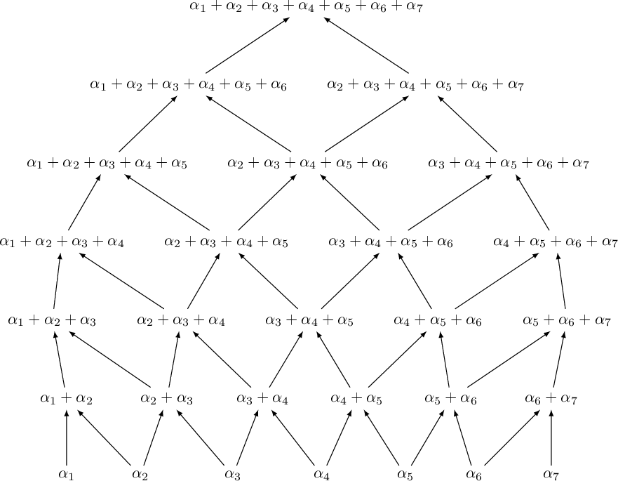
Here's another way to make this poset via algebra.

The triangle poset \leftrightarrow Type AnA_n positive root poset

W = RootSystem(["A",7]) PW7 = W.root_poset() show(PW7)

The box poset

\leftrightarrow Cartesian product of chains

P345 = Posets.ProductOfChains([3,4,5]) H345 = P345.hasse_diagram() show(H345, vertex_labels = False)
d3-based renderer not yet implemented
oi345 = P345.random_order_ideal() order_ideal_plot_colors(P345,set(oi345))

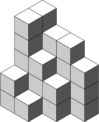
Order ideals in the 3D box are plane partitions!

Plane partitions are stacks of cubes in a corner.

PP345 = PlanePartitions([3,4,5]) ranPP345 = PP345.random_element() show(ranPP345)

Symmetry classes of plane partitions are coming! See trac ticket #28244.

A tetrahedral poset

PASM7 = Posets.TetrahedralPoset(7, 'green','yellow','blue','orange') plot(PASM7)
HASM7 = PASM7.hasse_diagram() show(HASM7, vertex_labels = False)
d3-based renderer not yet implemented
ASMoi = PASM7.random_order_ideal()
order_ideal_plot_colors(PASM7,ASMoi)

What's so special about this poset?

It's order ideals are in bijection with alternating sign matrices!

A7 = AlternatingSignMatrices(7) asm7 = A7.random_element() asm7
[ 0 0 0 0 1 0 0] [ 0 0 1 0 0 0 0] [ 0 1 -1 0 0 0 1] [ 1 -1 1 0 -1 1 0] [ 0 0 0 0 1 0 0] [ 0 1 0 0 0 0 0] [ 0 0 0 1 0 0 0]
A20 = AlternatingSignMatrices(20) asm20 = A20.random_element() asm20
20 x 20 dense matrix over Integer Ring
show(asm20)
(0010000000000000000000000000000010000000000000000100100010000000000100000000000000000011000001000000000000000001011011000000010001100000000000010100010101000000000001000100100001010101110100111000100000011110100000001100000000110000110100000000110001010101100010010100000010010000000000010110000100100000000000010011000000000000010111100000000100010001000000000000000110000100000000000000100000000000)\displaystyle \left(\begin{array}{rrrrrrrrrrrrrrrrrrrr} 0 & 0 & 1 & 0 & 0 & 0 & 0 & 0 & 0 & 0 & 0 & 0 & 0 & 0 & 0 & 0 & 0 & 0 & 0 & 0 \\ 0 & 0 & 0 & 0 & 0 & 0 & 0 & 0 & 0 & 0 & 0 & 0 & 1 & 0 & 0 & 0 & 0 & 0 & 0 & 0 \\ 0 & 0 & 0 & 0 & 0 & 0 & 0 & 0 & 0 & 1 & 0 & 0 & -1 & 0 & 0 & 0 & 1 & 0 & 0 & 0 \\ 0 & 0 & 0 & 0 & 0 & 0 & 0 & 1 & 0 & 0 & 0 & 0 & 0 & 0 & 0 & 0 & 0 & 0 & 0 & 0 \\ 0 & 0 & 0 & 0 & 0 & 0 & 1 & -1 & 0 & 0 & 0 & 0 & 0 & 1 & 0 & 0 & 0 & 0 & 0 & 0 \\ 0 & 0 & 0 & 0 & 0 & 0 & 0 & 0 & 0 & 0 & 0 & 1 & 0 & -1 & 1 & 0 & -1 & 1 & 0 & 0 \\ 0 & 0 & 0 & 0 & 0 & 1 & 0 & 0 & 0 & -1 & 1 & 0 & 0 & 0 & 0 & 0 & 0 & 0 & 0 & 0 \\ 0 & 0 & 0 & 1 & 0 & -1 & 0 & 0 & 0 & 1 & 0 & -1 & 0 & 1 & 0 & 0 & 0 & 0 & 0 & 0 \\ 0 & 0 & 0 & 0 & 0 & 1 & 0 & 0 & 0 & -1 & 0 & 0 & 1 & 0 & 0 & 0 & 0 & -1 & 0 & 1 \\ 0 & 1 & 0 & -1 & 1 & -1 & 0 & 1 & 0 & 0 & -1 & 1 & -1 & 0 & 0 & 0 & 1 & 0 & 0 & 0 \\ 0 & 0 & 0 & 1 & -1 & 1 & -1 & 0 & 1 & 0 & 0 & 0 & 0 & 0 & 0 & 0 & -1 & 1 & 0 & 0 \\ 0 & 0 & 0 & 0 & 0 & 0 & 1 & -1 & 0 & 0 & 0 & 0 & 1 & -1 & 0 & 1 & 0 & 0 & 0 & 0 \\ 0 & 0 & 0 & 0 & 1 & -1 & 0 & 0 & 0 & 1 & 0 & -1 & 0 & 1 & 0 & -1 & 1 & 0 & 0 & 0 \\ 1 & 0 & 0 & -1 & 0 & 1 & 0 & 0 & 0 & 0 & 0 & 0 & -1 & 0 & 0 & 1 & 0 & 0 & 0 & 0 \\ 0 & 0 & 0 & 0 & 0 & 0 & 0 & 1 & 0 & -1 & 1 & 0 & 0 & 0 & 0 & -1 & 0 & 0 & 1 & 0 \\ 0 & 0 & 0 & 0 & 0 & 0 & 0 & 0 & 0 & 0 & 0 & 1 & 0 & 0 & -1 & 1 & 0 & 0 & 0 & 0 \\ 0 & 0 & 0 & 0 & 0 & 0 & 0 & 0 & 0 & 1 & 0 & -1 & 1 & -1 & 1 & 0 & 0 & 0 & 0 & 0 \\ 0 & 0 & 0 & 1 & 0 & 0 & 0 & -1 & 0 & 0 & 0 & 1 & 0 & 0 & 0 & 0 & 0 & 0 & 0 & 0 \\ 0 & 0 & 0 & 0 & 0 & 0 & 0 & 1 & -1 & 0 & 0 & 0 & 0 & 1 & 0 & 0 & 0 & 0 & 0 & 0 \\ 0 & 0 & 0 & 0 & 0 & 0 & 0 & 0 & 1 & 0 & 0 & 0 & 0 & 0 & 0 & 0 & 0 & 0 & 0 & 0 \end{array}\right)

Back to rowmotion

oi7 = P7.random_order_ideal() show ( animate (list_of_order_ideal_plots(P7,set(oi7) )), delay = 80 )

There's another definition of rowmotion, in terms of:

Toggles

def order_ideal_plot_colors_toggles(myposet, elements, yellow_elements): order_ideal = myposet.subposet(myposet.order_ideal(elements)) order_filer = myposet.subposet(myposet.order_filter(myposet.order_ideal_complement_generators(order_ideal))) subposet = myposet.subposet(yellow_elements) order_ideal_color_dictionary = {} order_ideal_color_dictionary['blue'] = order_ideal order_ideal_color_dictionary['yellow'] = yellow_elements order_ideal_color_dictionary['red']= order_filer return myposet.plot(label_elements = False, element_colors = order_ideal_color_dictionary) def list_of_rowmotion_toggle_plots(myposet, orderideal): # starting = deepcopy(orderideal) output = [order_ideal_plot_colors(myposet, orderideal)] # while orderideal != starting: ranklist = [0..rank(myposet)] ranklist.reverse() for i in ranklist: ith_rank = [] for elem in myposet: if myposet.rank(elem) == i: ith_rank.append(elem) output.append(order_ideal_plot_colors_toggles(myposet, orderideal, ith_rank)) orderideal = myposet.order_ideal_toggles(Set(myposet.order_ideal(orderideal)),ith_rank) # print(ith_rank) # print(orderideal) output.append(order_ideal_plot_colors(myposet,orderideal)) output return output def list_of_rowmotion_orbit_toggle_plots(myposet, orderideal): starting = deepcopy(orderideal) output = list_of_rowmotion_toggle_plots(myposet, orderideal) orderideal = myposet.rowmotion(orderideal) while orderideal != starting: output.extend(list_of_rowmotion_toggle_plots(myposet, orderideal)) orderideal = myposet.rowmotion(orderideal) return output
show ( animate (list_of_rowmotion_toggle_plots(P7,set(oi7) )), delay = 40 )

Let's analyze this action.

How many elements are in each orbit? What is the order of the action?

sorted([len(orb) for orb in P7.rowmotion_orbits()])
[2, 4, 8, 8, 8, 8, 8, 8, 8, 8, 16, 16, 16, 16, 16, 16, 16, 16, 16, 16, 16, 16, 16, 16, 16, 16, 16, 16, 16, 16, 16, 16, 16, 16, 16, 16, 16, 16, 16, 16, 16, 16, 16, 16, 16, 16, 16, 16, 16, 16, 16, 16, 16, 16, 16, 16, 16, 16, 16, 16, 16, 16, 16, 16, 16, 16, 16, 16, 16, 16, 16, 16, 16, 16, 16, 16, 16, 16, 16, 16, 16, 16, 16, 16, 16, 16, 16, 16, 16, 16, 16, 16, 16, 16, 16]

The order of this action is 16. Looks like a rotation, but why?!

from sage.combinat.cyclic_sieving_phenomenon import * syt28 = StandardTableaux([8,8]) def sytpro(tab): return tab.promotion_inverse() sorted([len(orb) for orb in orbit_decomposition(list(syt28),sytpro)])
[2, 4, 8, 8, 8, 8, 8, 8, 8, 8, 16, 16, 16, 16, 16, 16, 16, 16, 16, 16, 16, 16, 16, 16, 16, 16, 16, 16, 16, 16, 16, 16, 16, 16, 16, 16, 16, 16, 16, 16, 16, 16, 16, 16, 16, 16, 16, 16, 16, 16, 16, 16, 16, 16, 16, 16, 16, 16, 16, 16, 16, 16, 16, 16, 16, 16, 16, 16, 16, 16, 16, 16, 16, 16, 16, 16, 16, 16, 16, 16, 16, 16, 16, 16, 16, 16, 16, 16, 16, 16, 16, 16, 16, 16, 16]
ransyt28 = syt28.random_element() show ( animate(list_of_bender_knuth_plots(ransyt28)), delay = 45 )
show ( animate( prolist ), delay = 40 )

Rowmotion on the Type An1A_{n-1} root poset

\leftrightarrow Toggling left-to-right on the Type An1A_{n-1} root poset

\leftrightarrow Promotion on 2×n2\times n standard Young tableaux

\leftrightarrow Rotation of the noncrossing matching

(first \leftrightarrow joint work with Nathan Williams)

(second \leftrightarrow is clear from the standard bijection)

(third \leftrightarrow is due to Dennis White)

There is a similar story for increasing tableaux and order ideals of the box poset.

inc345 = IncreasingTableau([[1,3,4,5],[2,4,7,8],[4,5,9,11]]) show ( animate(list_of_K_bender_knuth_plots(inc345,11)), delay = 40 )
show ( animate (list_of_rowmotion_toggle_plots(P345,set(oi345) )), delay = 40 )

Rowmotion on the [a]×[b]×[c][a]\times[b]\times[c] poset

\leftrightarrow K-Promotion on a×ba\times b increasing tableaux with entries at most a+b+c1a+b+c-1

(joint work with Kevin Dilks and Oliver Pechenik)

And let's look at alternating sign matrices

show ( animate (list_of_rowmotion_toggle_plots(PASM7,set(ASMoi) )), delay = 40 )
show( animate( [asm.to_fully_packed_loop() for asm in asm7.gyration_orbit()]), delay = 40)

Gyration on fully-packed loops (alternating sign matrices)

\leftrightarrow Rowmotion on the tetrahedral poset

(joint work with Nathan Williams)

(due to Ben Wieland)

show( animate( [asm.to_matrix() for asm in asm7.gyration_orbit()]), delay = 40)

For more on toggly-mathematics:

See my very recent talk at the 2020 BIRS Dynamical Algebraic Combinatorics workshop

http://www.birs.ca/events/2020/5-day-workshops/20w5164

For more on alternating sign matrix and plane partition code:

See my talk at the 2019 IMA workshop SageDays 99

https://www.ima.umn.edu/2018-2019/SW7.22-26.19/#schedule

Thanks to the organizers and the Sage community!