specialization_gb.ipynb

Kernel: Python 3 (system-wide)

This code goes along with a planned expository talk "The Description Problems for Ideals and Robots". Cf. slide 18 of presentation "Specialization of Grobner Bases II".

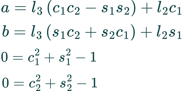
Let $\tilde{f}_i = F_if_i, \tilde{g_j} = G_jg_j.$

If $d\tilde{g_j} \in \tilde{I}$ for all $j$, then we can write

$$d\tilde{g}_j = \sum^{s}_{i = 1} \tilde{B}_{ji}f_i.$$

Dividing by $dG_j$,

$$\tilde{g}_j = \sum^{s}_{i = 1}(\frac{\tilde{B}_{ji}F_i}{dG_j})f_i = \sum^{s}_{i = 1} \tilde{B}_{ji}f_i,$$

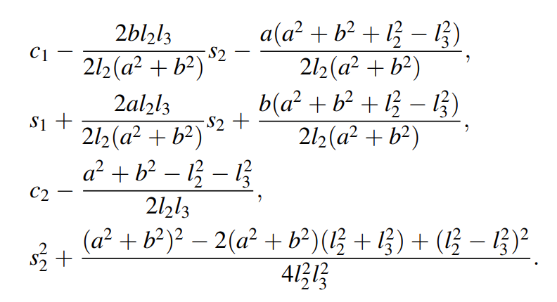
where the denominators of $\tilde{B}_{ji}$ are purely factors of $d$. We can form a Grobner basis for $I$ under the specialization $t \mapsto a \in k^m \ V(d).$ We check by:

1. Computing a Grobner basis $\tilde{G}$ for $\tilde{I}$ .

2. Dividing $d\tilde{j}$ by $\tilde{G}$.

Our subvariety $W \subseteq V$ exists by the vanishing of denominators $d = l_2l_3(a^2 + b^2)$. After clearing the denominators of our original Grobner Basis

we have new four new $\tilde{g}_j$ and check that $d \tilde{g}_j \in \tilde{I}$ :

R.<c1,s1,c2,s2,l2,l3,a,b>=PolynomialRing(QQ)
G=ideal(l3*c1*c2+l2*c1-l3*s1*s2-a,l3*c1*s2+l3*s1*c2+l2*s1-b,c1^2+s1^2-1,c2^2+s2^2
-1).groebner_basis()
d=l2*l3*(a^2+b^2)
tildeg1=l2*(a^2+b^2)*c1-b*l2*l3*s2-1/2*a*(a^2+b^2+l2^2-l3^2)
tildeg2=l2*(a^2+b^2)*s1+a*l2*l3*s2-1/2*b*(a^2+b^2+l2^2-l3^2)
tildeg3=l2*l3*c2-1/2*(a^2+b^2-l2^2-l3^2)
tildeg4=l2^2*l3^2*s2^2+1/4*((a^2+b^2)^2-2*(a^2+b^2)*(l2^2+l3^2)+(l2^2-l3^2)^2)
(d*tildeg1).reduce(G)
(d*tildeg2).reduce(G)
(d*tildeg3).reduce(G)
(d*tildeg4).reduce(G)

0

It does! Hence

(cf. slide 16 of presentation "The Inverse Kinematic Problem - Solving Our System II")

remains a Grobner basis for

(cf. slide 15 of presentation "The Inverse Kinematic Problem - Solving Our System I")

under all specializations in $\R[l_2, l_3, a, b] \ \textbf{V}(d)$. 🟪