Particle in a 1D Box.sagews

%md

# <img src="sagemathcloud_logo1.png" width="48"> Solving differential equations


- When solving differential equations it helps to specify which variables are real and which are positive using the **assume()** command.
- You need to specify the independent variable of your function.  In this case we specify that $\psi$ is a function of $x$.
- The differential equation is defined using the Python **def** method.
    - This creates a function which we can differential, integrate, or solve using the differential equation solver.
- Use **desolve()** to solve the differential equation.  The arguments of **desolve()** are the differential equation to solve, the dependent variable ($\psi$ in this case), and the independent variable x (specified using **ivar=x** to indicate the independent variable).

### Find general solution to Schrodinger's equation

The time-independent Schrodinger's equation in one dimension is $\frac{-\hbar^2}{2m} \frac{d^2}{dx^2}\psi(x) + V(x)\psi(x) = E \psi(x)$.  For an infinite square well of width $L$ the potential energy function is given by

\[ V(x) = \left\{ \begin{array}{cc} \infty & \text{if } x\ge L\\ 0 & \text{if } 0< x < L \\ \infty & \text{if } x \le 0 \end{array}\right. \]


<img src="particle_in_a_box.png" width=30%>

Note: To solve this differential equation we set the potential energy to zero inside the box and rearrange Schrodinger's equation so it has the form \(\frac{-\hbar^2}{2m} \frac{d^2}{dx^2}\psi(x) - E \psi(x) = 0\).

Solving differential equations

• When solving differential equations it helps to specify which variables are real and which are positive using the assume() command.

• You need to specify the independent variable of your function. In this case we specify that $\psi$ is a function of $x$.

• The differential equation is defined using the Python def method.

  • This creates a function which we can differential, integrate, or solve using the differential equation solver.

• Use desolve() to solve the differential equation. The arguments of desolve() are the differential equation to solve, the dependent variable ($\psi$ in this case), and the independent variable x (specified using ivar=x to indicate the independent variable).

Find general solution to Schrodinger's equation

The time-independent Schrodinger's equation in one dimension is $\frac{-\hbar^2}{2m} \frac{d^2}{dx^2}\psi(x) + V(x)\psi(x) = E \psi(x)$. For an infinite square well of width $L$ the potential energy function is given by

[ V(x) = \left{ $$\begin{array}{cc} \infty & \text{if } x\ge L\\ 0 & \text{if } 0< x < L \\ \infty & \text{if } x \le 0 \end{array}$$\right. ]

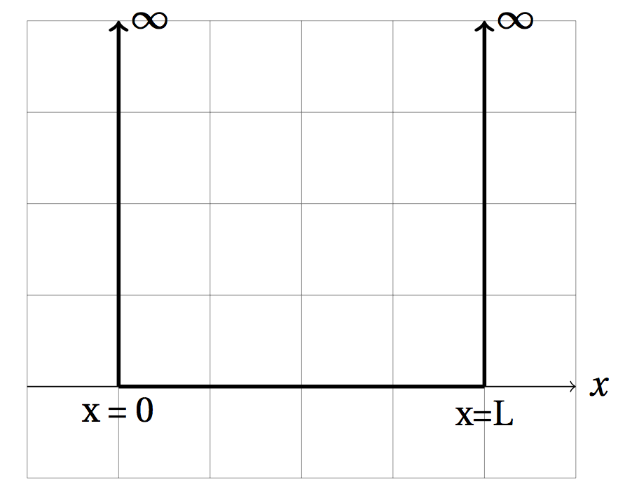
Note: To solve this differential equation we set the potential energy to zero inside the box and rearrange Schrodinger's equation so it has the form (\frac{-\hbar^2}{2m} \frac{d^2}{dx^2}\psi(x) - E \psi(x) = 0).

psi,m,L=var('psi,m,L')  #Declare wave function, mass, and box length as variables

Ener=var('Ener',latex_name=r'\mathcal{E}')  #Declare Ener as energy variable but will display a script E when using show() and pretty_print
hbar=var('hbar',latex_name=r'\hbar')  #Declares hbar as a variable and displays hbar symbol when using show() and pretty_print

assume(Ener,'real')   #Assume the variable Ener (the energy) only takes real values...
assume(Ener>0)   #... and assume the energy is greater than zero.  These are needed for desolve()

assume(m,'real')   #Assume the mass is real...
assume(m>0)     #... and positive.  If you don't make these assumptions you will get an error message asking if these variables are positive, negative, or zero

psi=function('psi')(x)   #To solve the differential equation we must tell SageMath that psi is a function called 'psi' with a single dependent variable


def f(psi):  #Define the equation to solve.
    return -hbar^2/(2*m)*diff(psi,x,2)-Ener*psi   #This is the differential equation to be solved

general_soln = desolve(f(psi)==0,psi,ivar=x)


pretty_print('The general solution to Schrodinger\'s equation is $\psi(x)=$', general_soln)

The general solution to Schrodinger's equation is $\psi(x)=$ $\displaystyle K_{2} \cos\left(\frac{\sqrt{2} \sqrt{{{\mathcal{E}}}} \sqrt{m} x}{{{\hbar}}}\right) + K_{1} \sin\left(\frac{\sqrt{2} \sqrt{{{\mathcal{E}}}} \sqrt{m} x}{{{\hbar}}}\right)$

Satisfying boundary conditions

The boundary conditions require that (\psi(x,t)) must be zero at the two walls. In other words, (\psi(x=0,t)=0) and (\psi(x=L,t)=0). Since (\sin(0)=0) and (\cos(0)=1), this means that (K_2=0). The boundary condition at (x=L) says that (K_1 \sin(\sqrt{2 \mathcal{E} m} x/\hbar) = 0) which is true if the argument of (\sin()) is an integer multiple of (\pi). Thus (\frac{\sqrt{2 m \mathcal{E}}L}{\hbar} = n \pi) for (n = 1, 2, 3, ...). To be consistent with previous notation we will set (A_0 = K_1). The wave function for the particle in a box is [\psi(x,t) = A_0 \sin(\frac{n \pi x}{L}).]

Integrating functions

• To integrate the function f(x) you can either use f(x).integrate(x) or integrate(f(x),x).

• For a definite integral, instead of just specifying the integration variable x you should specify the variable and the limits [x,0,L].

• Integrals frequently gives errors asking if a quantity is positive, negative, or zero. Use assume() commands to resolve this question.

Deterimine normalization constant

The integral of the probability density over some region of space gives the probability of finding the particle in that region. If we integrate over all possible places the particle might be, the total probability has to be 1 ( which corresponds to 100%). We can use this fact to find the normalization constant (A_0). In other words, by requiring (\int_0^L \psi^*(x,t) \psi(x,t) dx = 1) we can solve for (A_0).

A_0,n =var('A_0,n ')
assume(L,'real')  #Assume L is a real number
assume(L>0)  #Assume L is positive
assume(n,'integer')   #n must be an integer for a particle in an infinite square well - this is why we have quantization


psi_well(x,n)=A_0*sin(n*pi*x/L)   #Define the wave function

norm_int=integrate(psi_well*psi_well.conjugate(),[x,0,L])   #Integrate the probability density (psi* x psi) over the width of the well
pretty_print('The normalization integral gives ', norm_int)

answer=solve(norm_int==1,A_0)   #What value does A_0 need to have for a total probability of 1
pretty_print('The possible answers for $A_0$ are ', answer)

norm_const=answer[1].rhs()   #Select only the right hand side of the last term
pretty_print('We are only interested in the positive value  which is $A_0=$', norm_const)

psi_well(x,n)=psi_well(x,n).substitute(A_0=norm_const)  #Substitute our value for A_0 into the wave function
pretty_print('The equation for our wave function inside an infinite potential well is $\psi(x)=$', psi_well(x,n))

The normalization integral gives $\displaystyle n \ {\mapsto}\ \frac{1}{2} \, A_{0}^{2} L$

The possible answers for $A_0$ are [$\displaystyle A_{0} = -\frac{\sqrt{2}}{\sqrt{L}}$, $\displaystyle A_{0} = \frac{\sqrt{2}}{\sqrt{L}}$]

We are only interested in the positive value which is $A_0=$ $\displaystyle \frac{\sqrt{2}}{\sqrt{L}}$

The equation for our wave function inside an infinite potential well is $\psi(x)=$ $\displaystyle \frac{\sqrt{2} \sin\left(\frac{\pi n x}{L}\right)}{\sqrt{L}}$

More integration examples

Check orthogonality of infinite square well solutions

The wave functions for differing values of $n$ should be orthogonal to one another. This means that $\int_0^L \psi_n^*(x) \psi_m(x) dx = \delta_{mn}$

m=var('m')
assume(m,'integer')

probability_not_orthogonal=integrate(psi_well(x,n).conjugate()*psi_well(x,n),[x,0,L])  #Calculate for m=n
pretty_print(' If both wave functions have same n-value, then $\int_0^a\psi_n^*(x) \psi_n(x)dx$ = ', probability_not_orthogonal)


probability_orthogonal=integrate(psi_well(x,n).conjugate()*psi_well(x,m),[x,0,L])   #Calculate for m not equal to n
pretty_print(' If m is not equal to n, then $\int_0^a\psi_n^*(x) \psi_m(x)dx$ = ', probability_orthogonal)  #%todo: \ne or \neq not working

If both wave functions have same n-value, then $\int_0^a\psi_n^*(x) \psi_n(x)dx$ = $\displaystyle 1$

If m is not equal to n, then $\int_0^a\psi_n^*(x) \psi_m(x)dx$ = $\displaystyle 0$

2D plots of functions

• To plot a function (f(x)) vs. (x) from (x=0) to (x=2), use plot(f(x),[x,0,2])

• You can change the color of the line plotted by setting the color argument (e.g. color='black')

• Multiple graphs can be combined into a single plot window by adding the plot() commands together.

• Plots have various properties, such as line color, type of line, points plotted, titles, and axes labels that can be changed

• Use the show() command to display a plot

• When plotting functions with unspecified variables, set all variables to 1 using .substitute().

Plot wave function and probabilty density

The following commands demonstrate how to plot the wave function and probability densities for the first three lowest energy states of the 1D particle-in-a-box.

Since the potential energy (and thus the Hamiltonian) is symmetric about the center of the well (about the point (x=L/2)), the wave functions will either be symmetric or antisymmetric about (x=L/2). Since we haven't specified the length of the box we will set (L=1) for purposes of plotting.

psi_well_1(x)=psi_well(x,1).substitute(L=1)  #n = 1 ground state with L=1
psi_well_2(x)=psi_well(x,2).substitute(L=1)  #n = 2 first excited state with L=1
psi_well_3(x)=psi_well(x,3).substitute(L=1)  #n=3 second excited state with L=1

#The following three lines create plots of psi vs x
P1=plot(psi_well_1(x),[x,0,1],color='red',legend_label='n=1 State',title='First three wave functions of infinite well',axes_labels=['Position x','$\psi(x)$'])
P2=plot(psi_well_2(x),[x,0,1],color='blue',legend_label='n=2 State')
P3=plot(psi_well_3(x),[x,0,1],color='green',legend_label='n=3 State')


P=P1+P2+P3  #Combine graphs of first three states into a single object called 'P'...
P.show()  #... and display P on the screen

#The following three lines create plots of the probability density (psi*)psi vs x
P4=plot(psi_well_1(x)*psi_well_1(x).conjugate(),[x,0,1],color='red',legend_label='n=1 State',title='Probability density of first three states of infinite well',axes_labels=['Position x','|$\psi(x)|^2$'])
P5=plot(psi_well_2(x)*psi_well_2(x).conjugate(),[x,0,1],color='blue',legend_label='n=2 State')
P6=plot(psi_well_3(x)*psi_well_3(x).conjugate(),[x,0,1],color='green',legend_label='n=3 State')


PB=P4+P5+P6 #Combine the three graphs of probability density...
PB.show()   #...and show them on the screen

For you to try:

How does the number of peaks of the wave function compare to the value of n? How does the number of nodes of the wave function compare to the value of n? To help answer this question, plot the wave functions for the n=4 and n=5 states and see if they agree with your answer to these two questions. You can use psi_well(x,n) to define your wave functions.

#Insert your work here

Another example of integration

• SageMath will leave answers in exact form (e.g. 1/4 or pi) so to get numerical approximations you must use .n()

• You can specify how many digits are returned using .n(digits=3)

Probabilities to find the particle

The probability to find a particle between (x=a) and (x=b) is found by integrating the probability density over the region: [\int_a^b \psi^*(x) \psi(x) dx ]

What is the probability to find the particle somewhere in the box?

What is the probability of finding the particle in the left half of the box (between $x=0$ and $x=L/2$)?

What is the probability of finding the particle in the left quarter of the box (between $x=0$ and $x=L/4$)?

probability_somewhere=integrate(psi_well(x,1).conjugate()*psi_well(x,1),[x,0,L])

pretty_print("The probablity to find the particle somewhere is ", probability_somewhere)

probability_left_half=integrate(psi_well(x,1).conjugate()*psi_well(x,1),[x,0,L/2])

pretty_print("The probability to find the particle in the left half of the box between $x=0$ and $x=L/2$ is ", probability_left_half)

probability_left_quarter=integrate(psi_well(x,1).conjugate()*psi_well(x,1),[x,0,L/4])

pretty_print("The probability to find the particle in the left quarter of the box between $x=0$ and $x=L/4$ is ", probability_left_quarter, " = ", probability_left_quarter.n(digits=2) )

The probablity to find the particle somewhere is $\displaystyle 1$

The probability to find the particle in the left half of the box between $x=0$ and $x=L/2$ is $\displaystyle \frac{1}{2}$

The probability to find the particle in the left quarter of the box between $x=0$ and $x=L/4$ is $\displaystyle \frac{\pi - 2}{4 \, \pi}$ = $\displaystyle 0.091$

For you to try:

How do you think these three probabilities would differ for the $n=2$ state?

Calculate the probability for the particle to be somewhere inside the well, in the left half of the well, and in the left quarter of the well for the $n=2$ state. Compare these results to the answers for the $n=1$ state.

#Insert your work here

Expanding symbolic answers and obtaining numerical results

Calculating expectation values

• .expand() will distribute terms and expand powers in a symbolic expression

  • Note: When using .expand() on an express (rather than a variable), it helps to put parenthese around the expression.

    • This won't work 3*(x+y).expand() but (3*(x+y)).expand() will work.

• SageMath keeps results in exact form (e.g. $\sin(\pi/4)$ rather than $0.707$) but you can force SageMath to give an approximate answer using .n()

  • You can specify the number of digits the approximate result should have using .n(digits=3)

What is the expected value of the position of the particle $<x>$?

x_exp=integrate(psi_well(x,1).conjugate()*x*psi_well(x,1),[x,0,L]);x_exp  #Expecatation value of position <x>

x_exp.expand()  #Simplify the result by multiplying terms together

x_numeric=x_exp.substitute(L=1E-9)   #Set size of box to 1 nm
x_numeric.n()   #Force SageMath to compute numerical result
x_numeric.n(digits=3)   #You can specify the number of significant figures
pi.n(digits=7)   #Pi to seven places

def P(f):   #Definition of momentum operator
    return -i*hbar*diff(f,x)


p_exp=integrate(psi_well(x,1).conjugate()*P(psi_well(x,1)),[x,0,L])  #Expectation value of momentum <p>
p_exp

K_exp=integrate(psi_well(x,1).conjugate()*P(P(psi_well(x,1)))/(2*m),[x,0,L])  #Expectation value of kinetic energy <K>=<p^2>/2m
K_exp.show()

1/4*((2*pi^2 - 1)*L^2/pi^2 + L^2/pi^2)/L 1/2*L 5.00000000000000e-10 5.00e-10 3.141593 0

$\displaystyle \frac{\pi^{2} {{\hbar}}^{2}}{2 \, L^{2} m}$

Time-dependent behavior of the wave function and probability densities

psi_plot_1(x,t)=psi_well_1(x)*e^(i*pi^2/2*t)


plot_graph = [plot(psi_plot_1(x,t).real(),[x,0,1],color='red',ymin=-1.5,ymax=1.5) for t in sxrange(0,2,.1)]
a=animate(plot_graph)
a.show()

plot_graph_b = [plot(real(psi_plot_1(x,t)*psi_plot_1(x,t).conjugate()),[x,0,1],color='red',ymin=-2,ymax=2) for t in sxrange(0,2,.1)]
b=animate(plot_graph_b)
b.show()

For you to try:

Why does the wave function oscillate but the probability density does not? (Hint: the probability density involves multiplying the wave function by its complex conjugate)

Plot the wave function and probability density for the n=2 state and see if it displays the same behavior.

#Insert your work here

Animate plot of superposition of two states

psi_super(x,t)=psi_well_1(x)*e^(i*pi^2/2*t)+psi_well_2(x)*e^(i*4*pi^2/2*t)

plot_graph_c = [plot(psi_super(x,t).real(),[x,0,1],color='red',ymin=-2.5,ymax=2.5) for t in sxrange(0,2,.1)]
c=animate(plot_graph_c)
c.show()

plot_graph_d = [plot(real(psi_super(x,t)*psi_super(x,t).conjugate()),[x,0,1],color='red',ymin=0,ymax=6.5) for t in sxrange(0,2,.1)]
d=animate(plot_graph_d)
d.show()

%md

# For you to try:

Why does the probability density of the superposition state vary with time while the pure n=1 and n=2 states do not vary (Hint: The time dependence of the wave function is contained in the term \(e^{iE_n t/\hbar}\).  What happens to this time dependence when you calculate \(\psi^* \psi\) for the pure n=1 state or n=2 state? )

Plot the real part of a superposition of the n=1 and n=3 states $\psi_{super}(x,t)=\psi_{n=1}(x,t)+\psi_{n=3}(x,t)$.  Remember that the time dependency is $e^{iE_n t/\hbar}$ where $E_n=\frac{n^2\pi^2\hbar^2}{2mL^2}$ where we have assumed $\hbar=1$, $m=1$, and $L=1$ for plotting purposes.

For you to try:

Why does the probability density of the superposition state vary with time while the pure n=1 and n=2 states do not vary (Hint: The time dependence of the wave function is contained in the term (e^{iE_n t/\hbar}). What happens to this time dependence when you calculate (\psi^* \psi) for the pure n=1 state or n=2 state? )

Plot the real part of a superposition of the n=1 and n=3 states $\psi_{super}(x,t)=\psi_{n=1}(x,t)+\psi_{n=3}(x,t)$. Remember that the time dependency is $e^{iE_n t/\hbar}$ where $E_n=\frac{n^2\pi^2\hbar^2}{2mL^2}$ where we have assumed $\hbar=1$, $m=1$, and $L=1$ for plotting purposes.

#Insert your work here

Project Ideas and Problems to Solve

1. Normalize a 50/50 superposition of the n=1 and n=3 state where (\psi_{super}(x,t)=A_{norm}\left( \psi_{n=1}(x,t)+\psi_{n=3}(x,t)\right)). In other words, find the value of (A_{norm}) such that (\int_{-\infty}^{\infty}\psi^*(x,0) \psi(x,0) dx = 1).

2. Calculate [removed] for a particle in a superposition of the n=1 and n=3 states (\psi_{super}(x,t)=\psi_{n=1}(x,t)+\psi_{n=3}(x,t)).

3. Use the fact that the uncertainty of an observable is defined as (\Delta A = \sqrt{< A^2 > - < A >^2}) to find the uncertainty in the position and momentum for the first three states.

4. Repeat the previous question for the superposition of the n=1 and n=3 states.

︠de61fd7d-3903-4558-927a-feede2b403c9︠