Note: Hit Restart between cases
I've reused variable names for each case and failure to restart can cause results from a previous problem to cause issues with later solutions.
The three cases I've looked at are:
Wave function hitting a step potential with
Wave function hitting a step potential with
Wave function hitting a barrier potential with
Unbound States - Scattering and Tunneling
Solving the Schrodinger equation for unbound states is good practice for students in devloping an understanding of the wave function. It also gives students their first glimpse of quantum tunneling. This worksheet walks you through how to set up and solve the boundary conditions for the wave function and how to plot the graphs to gain deeper understanding.
The first case is a step potential with particle energy lower than the step potential height ()
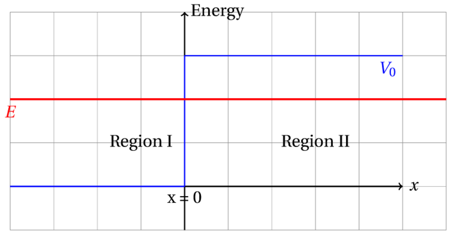
To solve this problem we assume a different wave function in each region but require that (1) the wave functions be continuous at the boundary and (2) the derivatives of the wave functions be continuous at the boundary. The two wave functions are:
[\psi_I(x) = A e^{ik_1 x} + B e^{-ik_1 x}]
and
[\psi_{II}(x) = C e^{k_2 x} + D e^{-ik_2 x}.]
The wave function must remain finite for all values of , which means that the first term in must be zero (i.e. )
The boundary conditions require:
[\psi_I(0) = \psi_{II}(0)]
and
[\frac{d \psi_I(x)}{dx}{x=0} = \frac{d \psi{II}(x)}{dx}_{x=0} .]
These equations are solved long-hand to demonstrate some of the symbolic manipulation functions of SageMath
.expand()Distributes and multiplies out all terms.combine()Collect terms over a common denominator.full_simplify()Runs numerous simplification routines
Assuming the particles are incident form the left, the coefficient is associated with the density of incoming particles. The reflection coefficient , which is the probability that a particle is reflected, can be found from the ratio of incoming to returning particles.
[R=\frac{BB^}{AA^} = \left| \frac{B}{A} \right|^2 ]
As expected, in this case we find that the reflection probability is , which means 100% of the particles are reflected back. However, the particles do penetrate into the classically forbidden region.
Plotting the wave function for the step potential
The step occurs at
The red part of the wave function shows where the particle tunnels into the step, which is classically forbidden
To animate the plot we add in the time dependence with for simplicity.

Animated plot of wave function
The following code creates an animation of the real part of the wavefunction to show how it changes in time.
For You To Try:
Plot the imaginary part of the wave function and animate it.
How does this graph differ from the real part?
Plot the probability density of the wave function
Step Potential:
For this next example we will find the wave function for a particle incident on a step potential with the particle energy larger than the step height.
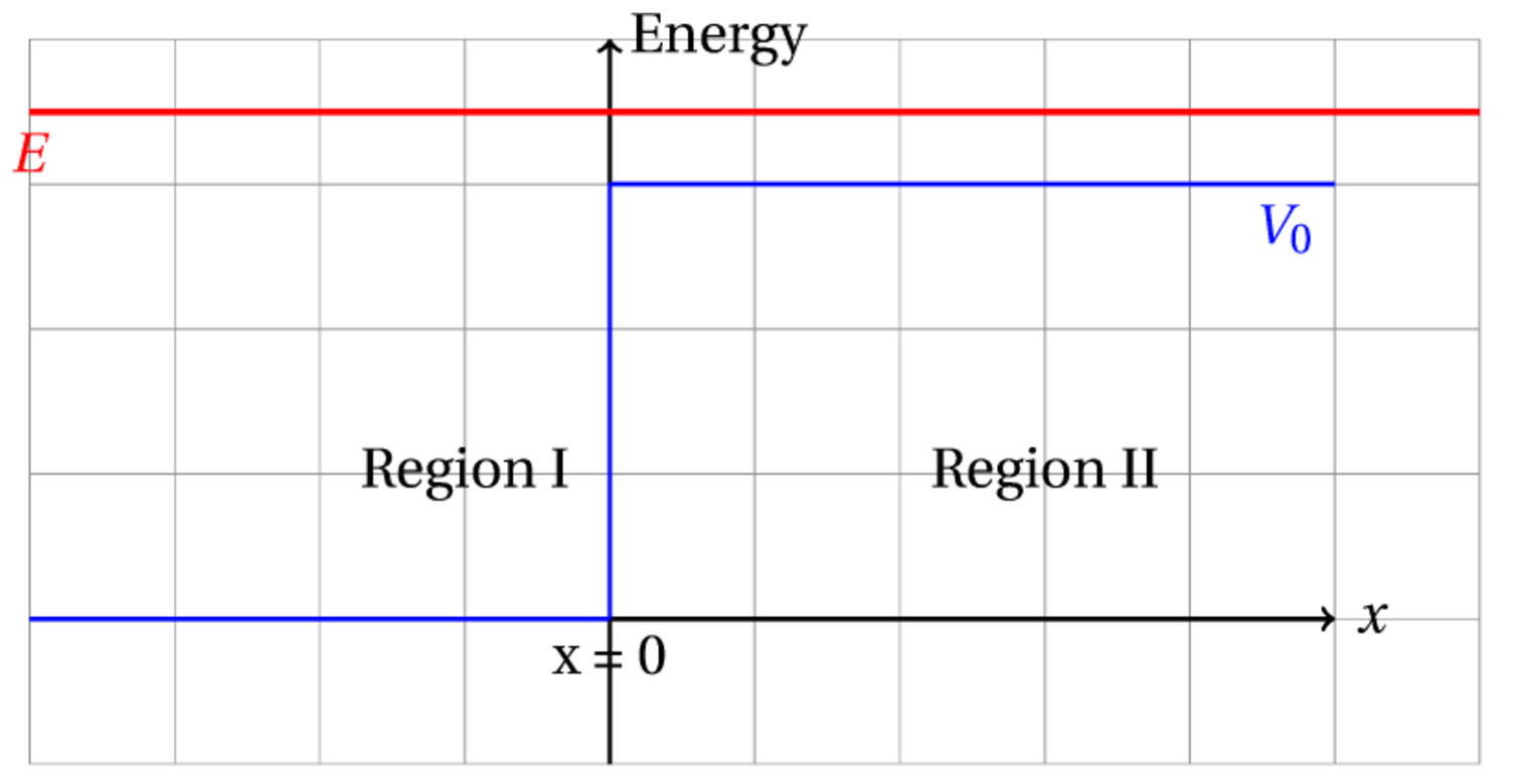
We expect that the particle reflection coefficient is no longer 100% in this case but classically we might not expect to see any reflection, but the graph at the bottom of the next cell shows that the reflection probability varies as a function of the energy difference between the particle and step potential.
The setup is the same as for the case except the wave function in region II is complex (and thus oscillatory).
The two wave functions are:
[\psi_I(x) = A e^{ik_1 x} + B e^{-ik_1 x}]
and
[\psi_{II}(x) = C e^{ik_2 x} + D e^{-ik_2 x}.]
If we assume there is no particles entering from the right then we must have .
The boundary conditions require:
[\psi_I(0) = \psi_{II}(0)]
and
[\frac{d \psi_I(x)}{dx}{x=0} = \frac{d \psi{II}(x)}{dx}_{x=0} .]
The function for the reflection probability and the transmission probability are plotted at the bottom of the next cell.

 Solve a system of equations
solve()returns a list of solutionsArguments of
solve()are a list of equations to satisfy and a list of variables to solve fore.g.
solve([x+y==1,x-y==3],[x,y])Note that equations must have double equals signs to work;
Barrier Tunneling
This example calculates the wave function for a particle hitting a barrier. It demonstrates that the particle does in fact tunnel through the barrier
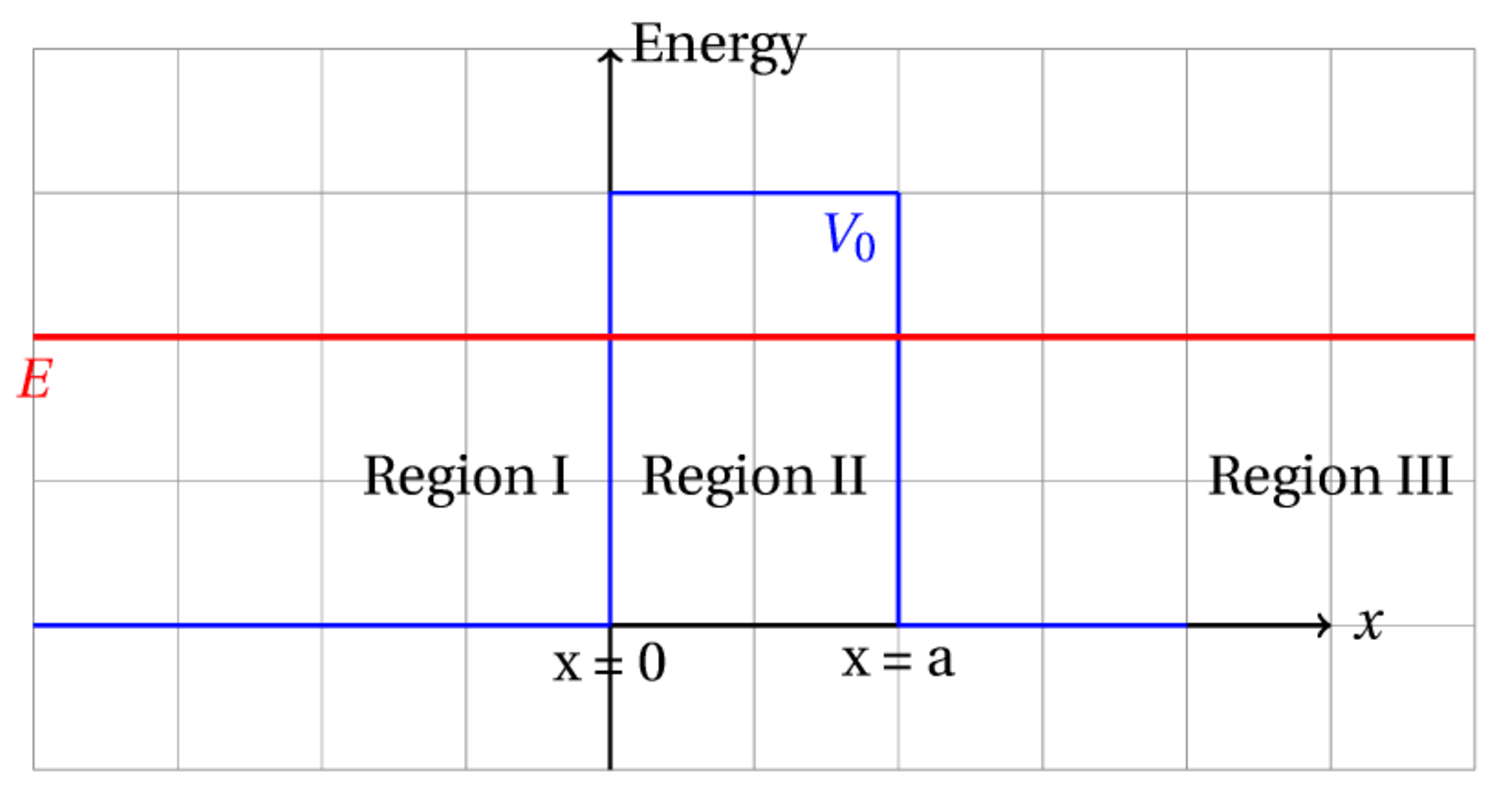
We now need to have wave functions in each of the three regions.
[\psi_I(x) = A e^{ik_1 x} + B e^{-ik_1 x}]
and
[\psi_{II}(x) = C e^{ik_2 x} + D e^{-ik_2 x}]
and
[\psi_{III}(x) = F e^{ik_1 x} + G e^{-ik_1 x}.]
With no particles incident from the right we can set .
The wave function and derivatives of the wave functions must be continuous at both boundaries. Rather than solving this set of equations long-hand, we'll use the solve() function to find , , , and .
The transmission probability is
[T=\frac{FF^}{AA^} = \left| \frac{F}{A} \right|^2.]
In this case the transmission probability through the barrier is non-zero, even though the particle should not be able to penetrate the barrier classically.

For You To Try
Type 'solve?' into the cell below and hit Shift+Enter to see the documentation for the
solve()commandUse
solve()to find the solutions to the equations:x+3y = 2
2y-4z=1
x-z=2
Projects and Problem Ideas
Calculate the reflection and transmisison probabilities for a barrier when E>V_0
Calculate the wave function and energy of a particle bound in a delta function well for E<0 (there is a single bound state)
Calculate the wave function for an unbound particle near a delta function well (E>0)