DUE-2016-05-20.sagews

Math 480 - Homework 6: numpy, scipy, and matplotlib

Due 6pm on May 20, 2016

HOMEWORK TOTAL: 60 POINTS

When you deduct points, state the reason.

Use your best judgement when assigning points. For example, if you feel their equation was just off by a slight typo, and it was worth 2 points, only deduct 0.5 or 1 point.

There are THREE problems. All problems are worth 20 points.

Problem 1 -- A comparison of 3d plots.

As you know, Sage has its own 3d plotting functionality built in. A significant drawback of Sage's 3d plotting (right now -- you could change this someday!) is that there is no support for generating publication quality pdf 3d plots using Sage's built-in 3d plotting. This problem is about several distinct ways to draw 3d plots using Sage.

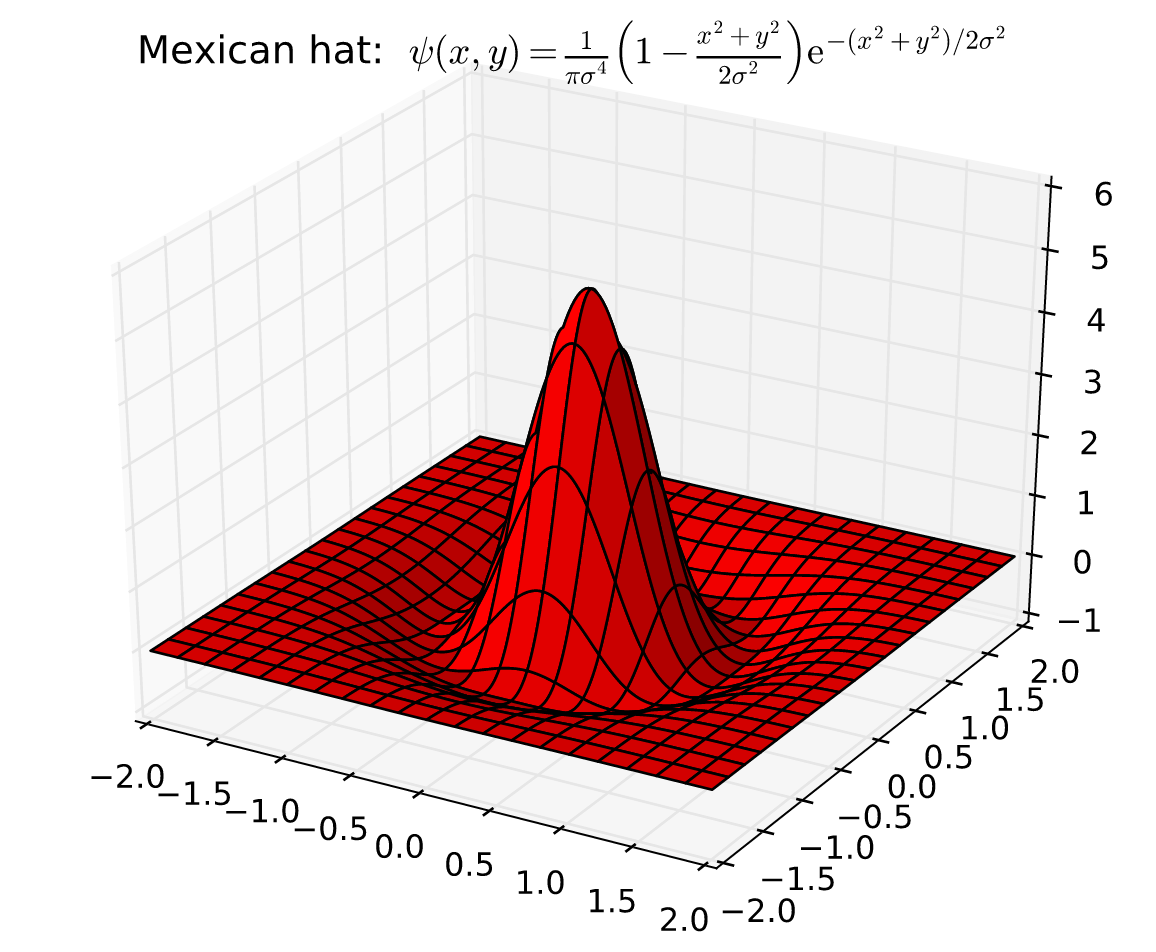
Your goal is to create several files -- hat1.png, hat2.png, and hat3.pdf -- containing plots of the bright red Mexican hat function $\displaystyle \psi(x,y) = \frac{1}{\pi\sigma^4}\left(1-\frac{x^2+y^2}{2\sigma^2}\right) \mathrm{e}^{-(x^2+y^2)/2\sigma^2}$
in the following ways, where $\sigma = 0.6$ and $-2\leq x, y \leq 2$. In each case, you should attempt to label the $z$-axis with the function definition (the formula right above) using nice-looking LaTeX.

20 Points Total

Part A : 5 pts
Part B : 5 pts
Part C : 10 pts

(Problem 1a.) Plotting using Sage:

• Use Sage's plot3d and text3d commands. Your text should NOT look good since Sage 3d plotting doesn't support LaTeX properly yet. The output of this problem should be the standard interactive 3d graph that you can rotate around. Don't forget to set the color and please set mesh=True in your plot3d command.

• Reminder: the surface should be red and the axes ranges are -2 to 2.

• Create a file called hat1.png that contains a picture of your 3d plot. The only current way to do this is to use your computer's screen capture functionality, then upload the resulting graphic using +New. So do that.

Part A (5 points)

Award:

• 2 points for a plot of the correct function. Needs correct $\mu$, bounds, and color for full points.
• 2 points for having some sort of attempted labeling using latex in text3d
• 1 point for having the an image of the plot in the folder

# Solution 1a.
f(x,y) = 1/(pi*0.6^4) *(1-(x^2 +y^2)/(2*0.6^2))*e^(-(x^2 +y^2)/(2*0.6^2))
P = plot3d(f,(-2,2),(-2,2), color='red', mesh=True)
g = P + text3d(r'z = \frac{1}{\pi\sigma^4}\left(1-\frac{x^2+y^2}{2\sigma^2}\right) \mathrm{e}^{-(x^2+y^2)/2\sigma^2}$', (2,2,2))
show(g)

3D rendering not yet implemented

(Problem 1b.) Using Sage 3d ray tracer.

• Render your Sage 3d graphic from above, but instead using Sage's Tachyon 3d raytracer, so you get a static png image in a file. Here is an example of how to render using Tachyon in a worksheet: icosahedron().save('icosahedron.png'); smc.file('icosahedron.png')

• The image file that you create should be called hat2.png and should end up in the current directory (same directory as your worksheet).

• Set the color of your plot to be red and make the range of the x and y axis be from -2 to 2.

• Label the plot with a beautiful latex formula... which will NOT actually work or look beautiful, due to shortcomings in Sage.

Part B (5 points)

Award:

• 1 point for a plot of the correct function. Needs correct $\mu$, bounds, and color for full points.
• 1 point for having some sort of attempted labeling using latex in text3d
• 2 points for using save() on the plot.
• 1 point for having the an image of the plot in the folder

# Solution 1b.
f(x,y) = 1/(pi*0.6^4) *(1-(x^2 +y^2)/(2*0.6^2))*e^(-(x^2 +y^2)/(2*0.6^2))
P = plot3d(f,(-2,2),(-2,2), mesh=True, color='red')
g = P + text3d(r'z = \frac{1}{\pi\sigma^4}\left(1-\frac{x^2+y^2}{2\sigma^2}\right) \mathrm{e}^{-(x^2+y^2)/2\sigma^2}$', (2,2,2))
g.save('hat2.png')
smc.file('hat2.png')

(Problem 1c.) Using plot_surface from matplotlib to plot the Mexican hat. This is more

difficult than the other approaches above... but it looks great!

• Look at the source code for the first example and change it appropriately.

• Remember to set the color of your plot to be red and make the range of the x and y axis be from -2 to 2.

• Remember to label the title with a beautiful latex formula...

• Remember to have matplotlib save the resulting image to the file hat3.pdf, in addition to displaying it.

Part A (10 points)

Award:

• 4 points for a plot of the correct function. Needs correct $\mu$, bounds, and color for full points.
• 4 points for having the fucntion labeled correctly in rendered LaTeX typesetting.
• 2 point for having a pdf of their image in the folder.

# Solution 1c.
%python
from mpl_toolkits.mplot3d import axes3d
import matplotlib.pyplot as plt
import numpy as np
def plot_surface():
    Y, X = np.mgrid[-2:2:200j, -2:2:200j]
    sigma = 0.6
    Z = 1/(np.pi * sigma**4) * (1 - (X**2 + Y**2)/(2*sigma**2))*np.exp(-1 * (X**2 + Y**2)/(2*sigma**2))

    fig  = plt.figure()
    ax = fig.add_subplot(111, projection='3d')
    ax.plot_surface(X, Y, Z, rstride=10, cstride=10, color='#ff0000')
    ax.set_title(r'Mexican hat:  $\psi(x,y) =  \frac{1}{\pi\sigma^4}\left(1-\frac{x^2+y^2}{2\sigma^2}\right) \mathrm{e}^{-(x^2+y^2)/2\sigma^2}$',
                 size='large')

plot_surface()
plt.show()
plt.savefig('hat3.pdf')

Problem 2 -- histograms and interact

The following function draws a histogram using Matplotlib. Try running it to verify that it works for you.

20 Points Total

Part A : 6 pts
Part B : 6 pts
Part C : 8 pts

def hist():
    import numpy as np
    import matplotlib.pyplot as plt

    mu, sigma = 100, 15
    x = mu + sigma * np.random.randn(1000)

    # the histogram of the data
    n, bins, patches = plt.hist(x, 50, normed=1, facecolor='g', alpha=0.75)

    plt.xlabel('Smarts')
    plt.ylabel('Probability')
    plt.title('Histogram of IQ')
    plt.text(60, .025, r'$\mu=100,\ \sigma=15$')
    plt.axis([40, 160, 0, 0.03])
    plt.grid(True)
    plt.show()

(Problem 2.a) Making your histogram function have inputs.

• Copy hist and make a new version that takes as input several relevant inputs: def hist_a(samples=1000, mu=100, sigma=15, bins=50, facecolor='g', alpha=0.75) so that you can instead call hist_a with different inputs.

• Call hist_a with the defaults, and also call it with every single input changed to something else in such as way that you can easily verify with your eyes that you correctly modified the body of the function to use the inputs to the function.

• The plot should correctly explain what mu and sigma are. Also, ensure that no matter what the inputs, the plot and text isn't partly cut off or missing from the figure.

Part A (6 points)

Award:

• 2 points for a function with correct defaults.
• 2 points for call to hist_a with input different from the defaults.
• 2 points for an explained $\mu$ and $\sigma$.

# Solution 2.a
def hist_a(samples=1000, mu=100, sigma=15, bins=50, facecolor='g', alpha=0.75):
    import numpy as np
    import matplotlib.pyplot as plt

    x = mu + sigma * np.random.randn(samples)

    # the histogram of the data
    n, bins, patches = plt.hist(x, bins, normed=1, facecolor=facecolor, alpha=alpha)

    plt.xlabel('Smarts')
    plt.ylabel('Probability')
    plt.title('Histogram of IQ')
    xmin, xmax, ymin, ymax = plt.axis()
    plt.text((xmax+2*xmin)/3, (ymax-ymin)/2, r'$\mu=%s,\ \sigma=%s$'%(mu, sigma))
    #plt.axis([mu-3*sigma, mu+3*sigma, 0, 0.03])  # no need!
    plt.grid(True)
    plt.show()

hist_a(samples=10000, mu=300, sigma=5, bins=500, facecolor='b', alpha=.5)

(Problem 2.b) Making your histogram function interactive.

• Make a copy of hist_a called hist_b and put @interact on the line before def hist_b(...) and evaluate.

• You will see input boxes for each of samples, mu, sigma, etc.

• Try editing some of them and hitting enter, and you'll see the output get updated as a result.

• Evaluate interact? in another worksheet (or cell) and look through some examples and docs involving @interact (you can also look at https://wiki.sagemath.org/interact for more examples.)

• Make it so each of the inputs to hist_b uses either a slider, dropdown, color selector, or buttons to select from a reasonable range of values (up to you).

• E.g., replace facecolor='g' by facecolor=Color('red') to get a color selector. You will have to figure out how to convert something like Color('red'), which is a Sage color, into something that is valid input as the facecolor to matplotlib! As usual, you will have to search docs and Google.

Part A (6 points)

If they continue errors from part 1, don't deduct the points again.

Award:

• 3 points for having a working interact
• 3 points for changing each of the inputs to either a slider, dropdown, color selector, or buttons.
• ie. it should NOT look exactly like the solution

# Solution 2.b
@interact
def hist_b(samples=1000, mu=100, sigma=15, bins=50, facecolor=Color('red'), alpha=0.75):
    import numpy as np
    import matplotlib.pyplot as plt

    x = mu + sigma * np.random.randn(samples)

    # the histogram of the data
    n, bins, patches = plt.hist(x, bins, normed=1, facecolor=facecolor.html_color(), alpha=alpha)

    plt.xlabel('Smarts')
    plt.ylabel('Probability')
    plt.title('Histogram of IQ')
    xmin, xmax, ymin, ymax = plt.axis()
    plt.text((xmax+2*xmin)/3, (ymax-ymin)/2, r'$\mu=%s,\ \sigma=%s$'%(mu, sigma))
    #plt.axis([mu-3*sigma, mu+3*sigma, 0, 0.03])  # no need!
    plt.grid(True)
    plt.show()

Interact: please open in CoCalc

(Problem 2.c) Adding a button to choose a distribution:

• Make a copy of hist_b above (with the interact) and call it hist_c. Add another button called dist, with values 'randn' and a at least 2 other distributions of your choice. Type np.random.[tab key] and read the documentation to find some other distributions (up to you which to add).

• Modify the code inside of hist_c so that it properly plots a histogram for sampling from the given distribution.

• In particular, you will have to change the line x = mu + sigma * np.random.randn(samples) to a more complicated if statement. (NOTE: You may just parameterize your distribution by mu and sigma still, even if that doesn't really make sense.)

Part A (8 points)

If they continue errors from part 1 and 2, don't deduct the points again.

Award:

• 4 points for correctly having selectors for the different distributions
• 4 points for having the distributions display correctly.
• You will have to look up what their distributions should look like.

# Solution 2.c
@interact
def hist_c(samples=1000, mu=100, sigma=15, bins=50, facecolor=Color('red'), alpha=0.75,
           dist=['randn', 'gumbel', 'pareto']):
    import numpy as np
    import matplotlib.pyplot as plt

    if dist == 'randn':
        x = mu + sigma * np.random.randn(samples)
    elif dist == 'gumbel':
        x = np.random.gumbel(mu, sigma, samples)
    elif dist == 'pareto':
        x = np.random.pareto(mu, samples)

    # the histogram of the data
    n, bins, patches = plt.hist(x, bins, normed=1, facecolor=facecolor.html_color(), alpha=alpha)

    plt.xlabel('Smarts')
    plt.ylabel('Probability')
    plt.title('Histogram of IQ')
    xmin, xmax, ymin, ymax = plt.axis()
    plt.text((xmax+2*xmin)/3, (ymax-ymin)/2, r'$\mu=%s,\ \sigma=%s$'%(mu, sigma))
    #plt.axis([mu-3*sigma, mu+3*sigma, 0, 0.03])  # no need!
    plt.grid(True)
    plt.show()

Interact: please open in CoCalc

Problem 3: Image compression with singular value decomposition

Read about singular value decomposition:

• https://en.wikipedia.org/wiki/Singular_value_decomposition.

• https://www.reddit.com/r/MachineLearning/comments/2b4nxd/eli5_singular_value_decomposition/cj1ua3j

There are 4 parts to this problem. Use the code below to assist you.

20 Points Total

Part A : 3 pts
Part B : 5 pts
Part C : 5 pts
Part D : 5 pts

# Working code to get you going... - you'll have to change the image name, and some parameters.
from scipy.ndimage import imread
import matplotlib.pyplot as plt
imgmat = imread("lion.jpg", flatten=True)
U, sigma, V = np.linalg.svd(imgmat)
k = 20
reconstimg = np.matrix(U[:, :k]) * np.diag(sigma[:k]) * np.matrix(V[:k, :])
lion = plt.imshow(reconstimg)
plt.show()

(Problem 3.a) Computing the SVD

• Upload your favorite image (preferably between 100 and 1000 pixels wide and tall)

• Use scipy.ndimage.imread to turn your image into a numpy matrix of grayscale entries. (When you call np.shape on this matrix, it should have the same dimensions as your image).

• Use numpy to compute the singular value decomposition (U, Sigma, and V) of your image.

• Use the first $k = 10$ vectors of the SVD to re-create the original matrix.

• Use matplotlib's imshow command (making sure to set cmap to "gray", otherwise you'll get a very colorful picture!) to display the new matrix, which is a compressed version of the original image.

Part A (3 points)

Award:

• 1 point for having uploaded an image into SMC
• 1 point for correctly reading in the image.
• 1 point for computing U, Sigma, and V

# Actual solution to 3.a (actual solution)
from scipy.ndimage import imread
import matplotlib.pyplot as plt
imgmat = imread("lion.jpg", flatten=True)
U, sigma, V = np.linalg.svd(imgmat)
k = 10
reconstimg = np.matrix(U[:, :k]) * np.diag(sigma[:k]) * np.matrix(V[:k, :])
lion = plt.imshow(reconstimg, cmap='gray')
plt.show()

(Problem 3.b) Examining the results

• Qualitatively, how well do you think the SVD compression with 10 vectors does at preserving the original image? Can you still tell what it's a picture of?

Part B (2 points)

Award:

• 2 points for answering the question completely

It does a decent job but the quality is terrible. It's still clear that it's a [lion], though.

(Problem 3.c) Further analysis

• What's the total combined size (number of entries) of the parts of U, Sigma and V that were used to reconstruct the image in part 1?

• What's the total size (number of entries) of the original matrix? What's the compression ratio?

Part C (10 points)

Award:

• 5 points for computing some values of uncompressed and compressed sizes.
• 5 points for computing the correct values based on the size of their image.

# Solution 3.c
# Original length * k + k + Original width * k
# Add a k due to the diagonal
compressed = 375 * 10 + 10 + 400 * 10
# Original size
uncompressed = 375 * 400
ratio = (uncompressed / compressed)
N(ratio)

19.3298969072165

(Problem 3.d) Messing around

• Try fiddling with the value of $k$ (using more or less of the SVD vectors to reconstruct the image).

• How many of the SVD vectors do you need to use before the compressed version is indistinguishable from the original?

Part D (5 points)

Award:

• 5 points for having a complete response which seems reasonable. (eg. They have an image that looks like the original)

# Solution 3.d
k = 25
reconstimg = np.matrix(U[:, :k]) * np.diag(sigma[:k]) * np.matrix(V[:k, :])
lion = plt.imshow(reconstimg, cmap='gray')
plt.show()