GitHub Repository: CloudPak-Outcomes/Outcomes-Projects
Path: blob/main/Db2-L3-Tech-Lab/IBM_Db2_Level_3.ipynb
¹⁹²⁸ views

Kernel: Python 3.10

Introduction

Data is the fuel that artificial intelligence (AI) engines run on. And databases often serve as the main repository for an organization's data. IBM has been a pioneer in data management technologies and advancements for decades. And a crucial part of this journey has been the invention of IBM Db2, a database built to address current data management needs, as well as provide an advantage as companies begin to incorporate AI into their workflows. Db2 databases are powered by AI to optimize and improve the data management process — AI-based features include a query optimizer that utilizes machine learning (ML), an adaptive workload manager that automatically adjusts concurrently running workloads to ensure the optimal number of queries are executed without compromising database stability, and built-in ML stored procedures that enable enterprises to learn from their data, at scale, without having to move it off-platform. Furthermore, Db2 is built for AI, ensuring users can effectively build AI models using popular programming languages like Python and R, as well as make them accessible through application programming interfaces (APIs) like representational state transfer (REST) APIs. All supported by enterprise-grade features like BLU Acceleration, massively parallel processing, and active compression, alongside robust security, highly available scalability (especially with pureScale technology), and disaster recovery.

This hands-on lab is designed to do several things:

Introduce you to some of the basic objects you will find in almost every Db2 database, as well as show you how to create and delete them
Show you how to create and execute some simple Structured Query Language (SQL) statements that can be used to store, modify, retrieve, and delete data in a Db2 database
Introduce you to some advanced Db2 topics such as the Db2 Explain facility, user defined functions, and SQL procedures
Illustrate how to build Python applications that interact with a Db2 database, regardless of whether the database is on-premises (created using IBM Db2 Community Edition) or in the Cloud (created under the Db2 "Lite" service on IBM Cloud).

Working with Jupyter Notebook

As you can see, this hands-on lab is provided in the form of a Jupyter Notebook. If you are unfamiliar with this technology, a Jupyter Notebook is an open source web application that enables users to create and share documents that contain narrative text, live code, equations, and rich outputs such as graphical visualizations. (Jupyter Notebook is maintained by Project Jupyter.) The name Jupyter comes from the core programming languages Jupyter Notebooks support: Julia, Python, and R. Jupyter ships with the IPython kernel, which enables users to write programs in Python, but there are currently over 100 other kernels that Jupyter Notebook supports.

The Jupyter Notebook framework contains several menu items and icons that enable users to interact with a notebook. The menu runs along the top of a Notebook just like menus do in other applications; the icons (buttons) are found just below the menu items. This introduction doesn't go into detail about each option available with every menu item. Instead, it will focus on just the two icons you will need to be familiar with to perform the exercises in this lab — these icons/buttons are emphasized in the following illustration:

The

icon (button) is used to save any changes you make to the notebook. Ctrl+s (Command+s on Mac) performs the same function.

The

icon (button) is used to execute the code — in our case Python — shown in a "Code" cell. Shift+Enter performs the same function.

If there are multiple code cells in a Notebook (as there are in this Notebook) and you run the cells in order, imports (external modules that are loaded into an application for use) and variables can be shared across cells. This makes it easy to separate out code into logical chunks without needing to reimport libraries or recreate variables or functions in each cell. (That being said, you will see some variables get recreated in each code cell in this lab — that's done to both reset the variable and to draw your attention to the variables that are used for each operation.)

When you select a code cell, you will notice that there are some square braces () beside the word In located at the top and just to the left of the cell. As you work your way through the Notebook, the square braces will be filled with a number that indicates the order in which each cell was ran. For example, if you run the first code cell found at the top of a Notebook, the square braces will be filled with the number 1. If you run the next code cell found after it, the square braces beside that cell will be filled with the number 2, and so on. While a code cell is being executed, the square braces will be filled with an asterisk (*).

How this lab is organized

The exercises found in this hands-on lab are organized as follows:

Section 1. Prepare the lab environment: Step 1. Set up the Jupyter Notebook environment; Step 2. Create a function that uses APIs in the ibm_db driver to execute SQL queries and retrieve/display query results; Step 3. Assign values to application variables that will be used to establish a database connection
Section 2. IBM Db2 basics: Step 1. Establish a database connection; Step 2. Query the database's system catalog; Step 3. Create a table named EMPLOYEE; Step 4. Insert a record into the EMPLOYEE table; Step 5. Add additional records to the EMPLOYEE table using a prepared INSERT statement with parameter markers; Step 6. Create a second table named DEPARTMENT and populate it; Step 7. Create a view named EMP_DEPT; Step 8. Change a record in the EMPLOYEE table; Step 9. Remove records from the EMPLOYEE table; Step 10. Create the tables that are used by the Db2 Explain facility ( Optional ); Step 11. Collect Explain data for a simple query ( Optional ); Step 12. Create an index named EMP_IDX; Step 13. Generate Explain data for the simple query again to see if the new index improves query performance ( Optional ); Step 14. Roll back and commit a transaction
Section 3. Advanced topics: Step 1. Create two user defined functions; Step 2: Invoke an SQL Scalar and an SQL Table user defined function; Step 3. Create an SQL procedure; Step 4: Invoke an SQL procedure
Section 4. Lab environment clean up: Step 1. Remove the tables used by the Db2 Explain facility ( Optional ); Step 2: Query the system catalog to see all the user-defined objects created in this lab; Step 3. Remove all user-defined objects created earlier from the database; Step 4. Query the system catalog again to confirm that all user-defined objects created in this lab have been deleted; Step 5. Terminate the database connection

NOTE: The following conventions are used whenever the syntax for a Db2 command or SQL statement is presented:

[ ]	:	Parameters or items shown inside brackets are required and *must* be provided.
< >	:	Parameters or items shown inside angle brackets are optional and do not have to be provided.
\|	:	Vertical bars indicate that one (and only one) item in the list of items presented can be specified.
, ...	:	A comma followed by three periods (ellipsis) indicate that multiple instances of the preceding parameter or item can be included in the Db2 command or SQL statement.

The following example illustrates each of these conventions:

Example:

REFRESH TABLE [ TableName , ... ]
< INCREMENTAL | NON INCREMENTAL >

In this example, you must supply at least one TableName value, as the brackets ( ) indicate, and you can provide more than one TableName value, as the comma and ellipsis ( , ... ) characters that follow the TableName parameter suggest. INCREMENTAL and NON INCREMENTAL are optional, as the angle brackets ( < > ) signify, and you can specify either one or the other, but not both, as the vertical bar ( | ) indicates.

Using IBM Db2 Community Edition with this hands-on lab

While this hands-on lab is set up to be ran with the Db2 "Lite" service on IBM Cloud, this Jupyter Notebook can be used with IBM Db2 Community Edition as well. IBM Db2 Community Edition is a special no-charge, full featured version of Db2 that enables data professionals to develop and deploy applications using any of the features and functionality found in in the latest release of IBM Db2. There are no limits on how long IBM Db2 Community Edition can be used, and unlike with the Db2 "Lite" service on IBM Cloud, there are no limits on the size of databases that can be created. However, there are limits on the number of cores and amount of memory supported: IBM Db2 Community Edition can be used with up to four processor cores and no more than 16 gigabytes (GB) of random access memory (RAM). One advantage of using IBM Db2 Community Edition for this lab is that the exercises labeled "Optional " can be executed — with the Db2 "Lite" service on IBM Cloud, the code for these exercises can be examined, but the code cells cannot be run.

To download a copy of IBM Db2 Community Edition, simply go to the IBM Db2 web site (which can be found here: IBM Db2 Database) and click on the “Try it on premises →” button shown on the page. After completing and submitting the form presented, you will be re-directed to the IBM Db2 Download Center web site. Once there, select the “Download” link that corresponds to the operating system you plan to install IBM Db2 Community Edition on. When the file has finished downloading, refer to the IBM Db2 documentation for instructions on how to install and configure the IBM Db2 Community Edition software. (Instructions for installing Db2 Version 11.5 can be found here: Db2 servers and IBM data server clients. A Bash shell script that streamlines and automates the installation process on Ubuntu Linux is available here: db2_env_setup.sh — right-click on the link and select "Save Link As..." to download this file.)

IMPORTANT: If you do not complete this lab in a single sitting, you must re-run all the exercises in Section 1 and the first two exercises in Section 2 before you attempt to pick back up where you left off!

Section 1. Prepare the lab environment

Step 1. Set up the Jupyter Notebook environment

Overview:

Before you can begin interacting with an IBM Db2 database using Python or Jupyter Notebook, there are some basic steps you must perform. These steps include:

Downloading and installing the ibm_db Python database interface driver for IBM Db2, IBM Informix, IBM Db2 for iSeries(AS400) and IBM Db2 for z/OS servers.
Loading (importing) the ibm_db driver into the Python application or Jupyter Notebook.
Loading any additional external Python modules needed into the Python application or Jupyter Notebook.
Defining any variables that will be used to supply information to, or obtain infromation from application programming interfaces (APIs) in the ibm_db driver. (These APIs are used to do things like establish a connection to a database, submit a query for execution, retreive query results, and so forth.)

Execute the code:

The code in the next "cell" performs all but the last of the tasks just identified — the task of defining variables will be performed, when necessary, throughout the remaining exercises in this lab.

Select the code cell below and carefully read through the comments (i.e., the text that begins with a # character). This will help you understand the actions the code performs.

When you are ready, click on the

button or press Shift+Enter to execute the code.

In [ ]:

#----------------------------------------------------------------------------------------------#
# Set Up The Jupyter Notebook Environment                                                      #
#----------------------------------------------------------------------------------------------#

#----------------------------------------------------------------------------------------------#
# Download And Install The ibm_db Driver Package                                               #
#   NOTE: This only needs to be preformed once in a runtime environment and may have already   #
#   been done. If so, it is not harmful to attempt to install the package again, as subsequent #
#   attempts will simply state that the package requirement has already been satisfied.        #
#----------------------------------------------------------------------------------------------#
print()
!python3 -m pip install ibm_db

#----------------------------------------------------------------------------------------------#
# Load The Appropriate Python Modules                                                          #
#----------------------------------------------------------------------------------------------#
import sys                        # Provides Information About Python Interpreter Constants,
                                  # Functions, And Methods
from io import StringIO           # Implements A File-Like Class That Reads And Writes A String
                                  # Buffer (i.e., A Memory File)
from IPython import get_ipython   # Simple Function To Call To Get The Current Interactive Shell
                                  # Instance
import ibm_db                     # Contains The APIs Needed To Work With Db2 Databases

#----------------------------------------------------------------------------------------------#
# Define A Python Class Named ipynb_Exit()                                                     #
#----------------------------------------------------------------------------------------------#
#  CLASS NAME:  ipynb_Exit()                                                                   #
#  PURPOSE:     This class contains the programming logic needed to allow Python "exit()"      #
#               functionality to work without raising an error or stopping the Jupyter         #
#               Notebook kernel in the event the exit() function is called.                    #
#----------------------------------------------------------------------------------------------#
class ipynb_Exit(SystemExit):
    """Exit Exception for IPython. Exception Temporarily Redirects stderr To Buffer."""

    #------------------------------------------------------------------------------------------#
    #  FUNCTION NAME:  __init()__                                                              #
    #  PURPOSE:        This method initializes an instance of the ipynb_Exit class.            #
    #------------------------------------------------------------------------------------------#
    def __init__(self):
        sys.stderr = StringIO()      # Redirect sys.stderr to a StringIO (memory buffer) object.

    #------------------------------------------------------------------------------------------#
    #  FUNCTION NAME:  __del()__                                                               #
    #  PURPOSE:        This method cleans up when an instance of the ipynb_Exit class is       #
    #                  deleted.                                                                #
    #------------------------------------------------------------------------------------------#
    def __del__(self):
        sys.stderr = sys.__stderr__  # Restore sys.stderr to the original values it had at
                                     # the start of the program.

#----------------------------------------------------------------------------------------------#
# Define A Python Function Named customExit()                                                  #
#----------------------------------------------------------------------------------------------#
#  FUNCTION:  customExit()                                                                     #
#  PURPOSE:   This function is used to define a customized exit process.                       #
#----------------------------------------------------------------------------------------------#
def customExit(returnCode=0):
    if returnCode == 0:
        ipynb_Exit()
    else:
        raise ipynb_Exit

#----------------------------------------------------------------------------------------------#
# If An IPython Application (i.e., A Jupyter Notebook) Calls The "exit() Function, Call A      #
# Customized Exit Routine So The Jupyter Notebook Will Not Stop Running - Otherwise, Call The  #
# Default Exit Routine                                                                         #
#----------------------------------------------------------------------------------------------#
if get_ipython():    
    exit = customExit                # Rebind To The Custom Exit Function
else:
    exit = exit                      # Just Call The Exit Function

#----------------------------------------------------------------------------------------------#
# Display A Status Message Indicating This Work Is Complete                                    #
#----------------------------------------------------------------------------------------------#
print("\nAll initialization work is complete!\n")

Step 2: Create a function that uses APIs in the ibm_db driver to execute SQL queries and retreive/display query results

Overview:

Structured Query Language (SQL) is a standardized language that is used to work with database objects and the data they contain. Using SQL, it's possible to define, alter, and delete database objects, as well as add data to, change data in, and retrieve or remove data from any objects created. Because SQL is non-procedural by design, it is not considered an actual programming language even though, like other programming languages, it has a defined syntax and its own set of language elements. Consequently, applications that utilize SQL are are typically built by combining the decision and sequence control of a high-level programming language — in our case, Python — with the data storage, manipulation, and retrieval capabilities SQL provides.

SQL statements are frequently categorized according to the function they're designed to perform:

Embedded SQL Application Construct statements: Used for the sole purpose of constructing embedded SQL applications. (Applications written with the C programming language frequently use these statements.)
Data Control Language (DCL) statements: Used to grant and revoke authorities and privileges needed for Db2 instance management and data access.
Data Definition Language (DDL) statements: Used to create, alter, and delete database objects.
Data Manipulation Language (DML) statements: Used to store data in, modify data in, retrieve data from, and remove data from select database objects.

Because many of the exercises found in this lab focus on constructing and executing DDL and DML statements, the database used will be queried often to ensure that operations desired are performed as expected. Rather than repeat the Python code needed to execute a query, retreive the results, and display the information obtained every time a query is executed, the code in the following cell will encapsulate this work in a Python function that can be called whenever a query needs to be executed.

With Python and Jupyter Notebook, application programming interfaces (APIs) in the ibm_db Python database interface driver are used to submit SQL statements to a Db2 database for processing, as well as retreive results. The APIs used in the code in the following cell include:

•	ibm_db.exec_immediate( )	:	Used to prepare and execute an SQL statement, using values supplied for parameter markers that were coded in the statement (if there are any), immediately.
•	ibm_db.stmt_errormsg( )	:	Used to return an SQLCODE and corresponding error message that explains why an attempt to return an IBM_DBStatement object from an ibm_db.prepare( ), ibm_db.exec_immediate( ), or ibm_db.callproc( ) API call was unsuccessful; can also be used to return an SQLCODE and error message that identifies why the last operation using a IBM_DBStatement object failed.
•	ibm_db.fetch_tuple( )	:	Used to retrieve a row (record) from a result set and copy its data to a Python tuple. Depending on how it is called, it can advance a cursor to the next row in a result set and copy the data for that row into a tuple. Or, it can be used to retrieve the data for a specific row — provided a keyset driven, dynamic, or static cursor is used to traverse the result set. In either case, the value for the first column in the row will be stored in the first position of the tuple (index position 0), the second column will be stored in the second position (index position 1) and so on. .

You can learn more about the APIs that are available with the ibm_db Python interface driver here: IBM Db2-Python and here: ibmdb/python-ibmdb APIs.

Execute the code:

Select the code cell below and carefully read through the comments. This will help you understand the operations the function performs.

When you are ready, click on the

button or press Shift+Enter to execute the code.

In [ ]:

#----------------------------------------------------------------------------------------------#
# Define A Python Function Named runQuery()                                                    #
#----------------------------------------------------------------------------------------------#

#----------------------------------------------------------------------------------------------#
#  FUNCTION NAME:  runQuery()                                                                  #
#  PURPOSE:        This function attempts execute an SQL query (SELECT statement) and then     #
#                  display any results obtained.                                               #
#                                                                                              #
#  PARAMETERS:     dispInfo   - A value that indentifies what information is to be displayed   #
#                                 (0 - Display everything; 1 - Display records and row count;  #
#                                  2 - Display records only)                                   #
#                  sqlStmt    - The SQL query statement to be executed                         #
#                  colHeaders - A Python tuple containing display column header information    #
#                  colWidths  - A Python tuple containing display column width information     #
#                                                                                              #
#  RETURNS:        True       - The query was executed and the results were displayed          #
#                  False      - The query was not executed or the results were not displayed   #
#----------------------------------------------------------------------------------------------#
def runQuery(dispInfo, sqlStmt, columnHeaders, columnWidths):
    
    # Define And Initialize The Appropriate Variables
    resultSet = False                        # Pointer To A Query Result Set
    errorMsg = ""                            # Detailed Error Information
    noData = False                           # No Data Found Flag
    firstPass = True                         # First Pass Through Record Display Loop Flag
    dataRecord = False                       # Data Record
    numColumns = len(columnHeaders)          # Number Of Values In The Column Headers Tuple
    numRows = 0                              # Number Of Records (Rows) Retreived 
    tupIndx = 0                              # Tuple Index
    dataValue = ""                           # Data Value String
    newValue = ""                            # Trimmed Data Value String
    
    # If The dispInfo Variable Is Set To 0, Display The SQL Statement That Is To Be Executed,
    # Along With A Message That The Statement Is Being Executed
    if dispInfo == 0:
        print("\nExecuting the following SQL statement:\n\n" + sqlStmt)
        
    # Execute The SQL Statement Provided By Calling The ibm_db.exec_immediate() API
    # (This API Prepares And Executes An SQL Statement In A Single Step)
    try:
        resultSet = ibm_db.exec_immediate(connectionID, sqlStmt)
    except Exception:
        print("\nERROR: Unable to execute the SQL statement specified.\n")    
        pass

    # If The SQL Statement Could Not Be Executed, Display An Error Message And Return
    # FALSE To The Calling Function (Call The ibm_db.stmt_errormsg() API To Obtain
    # Detailed Error Information)
    if resultSet == False:
        errorMsg = ibm_db.stmt_errormsg()
        print(errorMsg + "\n")
        return(False)       
        
    # Otherwise, Print A Blank Line And Begin Processing Any Records Retreived
    else:
        print()
       
    # As Long As There Are Records In The Result Set Produced, ...
    while noData == False:

        # Retrieve A Record And Store Its Values In A Tuple By Calling
        # The ibm_db.fetch_tuple() API
        try:
            dataRecord = ibm_db.fetch_tuple(resultSet)
        except:
            print("ibm_db.fetch_tuple() returned an error.\n")
            pass

        # If A Record Could Not Be Retrieved Or If No Record Was Found, 
        # Set The "No Data" Flag To TRUE To Exit The while() Loop
        if dataRecord == False:
            noData = True
            
            # If This Is The First Pass Through The while() Loop,
            # Display A "No Records Found" Message And Exit The Loop
            if firstPass == True:
                print("No records found.")
                break

        # Otherwise, Display The Appropriate Information
        else:
            
            # If This Is The First Pass Through The while() Loop, ...
            if firstPass == True:
                
                # If The dispInfo Variable Is Set To 0 Display A "Query Results" Header Label
                if dispInfo == 0:
                    print("Query results:\n")

                # Display The Column Headers Provided In The columnHeaders Tuple - Left Justify
                # The Text And Make Each Column The Width Specified In The columnWidths Tuple
                for tupIndx in range(numColumns):
                    print(f'{columnHeaders[tupIndx]:<{columnWidths[tupIndx]}}', end="")
                    print("  ", end="")      # Space Between Column Header Values           
         
                # Terminate The Line And Display Column Header/Value Dividing Lines Just Below
                # The Column Headers
                print()
                for tupIndx in range(numColumns):
                    print(f'{"":-<{columnWidths[tupIndx]}}', end="")
                    print("  ", end="")       # Space Between Column Header Dividing Lines  
                    
                # Terminate The Line And Set The "First Pass" Flag To FALSE So Header
                # Information Will Not Be Displayed Again
                print()
                firstPass = False
            
            # Format And Display The Data For Each Record Retreived
            for tupIndx in range(numColumns): # For Every Column In The Record, ...
                
                # Copy The Data Value Into A Character String Variable And
                # Remove Any Trailing Space Characters Found
                dataValue = "{}".format(dataRecord[tupIndx])
                newValue = dataValue.rstrip()
 
                # If The Data Value IS NOT A Character String, Display It Right Justified,
                # Using The Width Specified In The columnWidths Tuple 
                if type(dataRecord[tupIndx]) != str:
                    print(f'{newValue:>{columnWidths[tupIndx]}}', end="")
    
                # Otherwise (The Data Value Is A Character String), ...
                else:
        
                    # If The Character String Only Contains Alphabetical Characters,
                    # Display It Left Justified, Using The Width Specified In The
                    # columnWidths Tuple
                    if newValue.isalpha() == True:                
                        print(f'{newValue:<{columnWidths[tupIndx]}}', end="")
        
                    # Otherwise, See If The Character String Contains A Space Or
                    # Underscore Character (If It Does, isalpha() Will Return False)
                    else:
                        
                        # If The Character String Contains A Space Or Underscore Character,
                        # Display The Character String Left Justified, Using The Width
                        # Specified In The columnWidths Tuple
                        if (" " in newValue or "_" in newValue) == True:
                            print(f'{newValue:<{columnWidths[tupIndx]}}', end="")
                                                    
                        # Otherwise, Display The Character String Right Justified, Using 
                        # The Width Specified In The columnWidths Tuple
                        else:
                            print(f'{newValue:>{columnWidths[tupIndx]}}', end="")
                
                # Add Spaces Between This Column Value And The Next 
                print("  ", end="")           # Space Between Column Values 
          
            # Terminate The Line And Increment The Records (Rows) Counter
            print()
            numRows = numRows + 1

    # If The dispInfo Variable Is Set To 1 And Records Were Retreived,
    # Display The Number Found
    if dispInfo <= 1 and firstPass == False:
        print("\nNumber of records (rows) found:", numRows)

    # Return TRUE To The Calling Function
    return(True)

# Display A Status Message Indicating The runQuery() Function Has Been Defined
print("\nA function named runQuery() has been defined!\n")

Step 3. Assign values to application variables that will be used to establish a database connection

Overview:

Before operations can be performed against an IBM Db2 database, a connection to the database must first be established. To do this, you need information about the database environment such as the database's name or alias, the host name or IP address of the database server, and the port number Db2 uses for TCP/IP communications. You also need appropriate authorization credentials, which typically consist of a user or authentication ID and a corresponding password. Instructions on how to obtain this information are provided in the main guide for this lab.

Execute the code:

Once you have collected the information needed, perform these steps to assign it to the application variables that will be used later to establish a database connection:

Select the appropriate code cell below and assign values to the dbName, hostName, portNum, userID, and passWord application variables. If the database you are using is provided through the Db2 "Lite" service on IBM Cloud, modify the code in the cell immediately below the heading Step 3a: Connect to a remote, Db2 on Cloud database. On the other hand, if you are using a local database that was created with IBM Db2 Community Edition (or some other Db2 Edition), modify the code in the the cell immediately below the heading Step 3b: Connect to a local, on-premises Db2 database.

Click on the

button or press Ctrl+s (or command+s on Mac) to save your changes.

When you are ready, click on the

button or press Shift+Enter to execute the code.

IMPORTANT: Only execute the code in the cell below the heading Step 3a: or Step 3b: — DO NOT EXECUTE THE CODE IN BOTH CELLS!!!

Whenever new values are assigned to the variables in the cell below, the code must be saved and re-executed. Otherwise, the code in the code cells that follow may not execute correctly.

Step 3a: Connect to a remote, Db2 on Cloud database

In [ ]:

#----------------------------------------------------------------------------------------------#
# Initialize All User-Specific Connection Variables - Db2 on Cloud Database                    #
#   IMPORTANT: UPDATE WITH VALUES FROM YOUR OWN ENVIRONMENT, AS PER LAB INSTRUCTIONS.          #
#----------------------------------------------------------------------------------------------#

# Define And Initialize The Appropriate Variables
dbName = "bludb"
userID = "replace-with-your-userID"
passWord = "replace-with-your-password"
hostName = "replace-with-your-hostname"
portNum = "replace-with-your-port-number"

secureComm = True              # Use SSL (Secure Sockets Layer) Communication

# Display A Status Message Indicating This Work Is Complete
print("\nUser-specific connection variable initialization work complete!\n")

Step 3b: Connect to a local, on-premises Db2 database

In [ ]:

#----------------------------------------------------------------------------------------------#
# Initialize All User-Specific Connection Variables - Local Db2 Database                       #
#   IMPORTANT: UPDATE WITH VALUES FROM YOUR OWN ENVIRONMENT, AS PER LAB INSTRUCTIONS.          #
#----------------------------------------------------------------------------------------------#

# Define And Initialize The Appropriate Variables
dbName = "replace-with-your-db-name"       # The Alias For The Db2 Database
userID = "replace-with-your-userID"        # The Instance User ID
passWord = "replace-with-your-password"    # The Password For The Instance User ID
hostName = "replace-with-your-hostname"    # The Host Name
portNum = "replace-with-your-port-number"  # The TCP/IP Port Number That Receives Db2 Connections
                                           # On Db2 11.5.5 and older, the default port number
                                           #  is 50000 (Non-SSL) or 50001 (SSL).
                                           # On Db2 11.5.6 and newer, the default port number
                                           #  is 25000 (Non-SSL or 25001 (SSL).
secureComm = False              # Do NOT Use SSL (Secure Sockets Layer) Communication

# Display A Status Message Indicating This Work Is Complete
print("\nUser-specific connection variable initialization work complete!\n")

Section 2. IBM Db2 basics

Step 1: Establish a database connection

Overview:

As mentioned earlier, before anything can be done with a Db2 database, a connection to the database must first be established. With Python and Jupyter Notebook, the ibm_db.connect( ) API is typically used to perform this task. This API utilizes a connection string that has the following format:

DRIVER={IBM DB2 ODBC DRIVER};ATTACH=connType;DATABASE=dbName;HOSTNAME=hostName;PORT=portNum;PROTOCOL=TCPIP;SECURITY=SSL;UID=userName;PWD=passWord

where:

•	connType	:	Specifies whether a connection is to be made to Db2 server (`TRUE`) or a Db2 database (`FALSE`).
•	dbName	:	The name of the Db2 server or database the connection is to be made to.
•	hostName	:	The host name or IP address of the Db2 server — as it is known to the TCP/IP network — the connection is to be made to.
•	portNum	:	The port number that receives Db2 connections on the server the connection is to be made to.
•	userName	:	The user name/authorization ID that is to be used for authentication when the connection is established.
•	passWord	:	The password that corresponds to the user name/authorization ID specified in the *userName* parameter.

NOTE: When working with a local Db2 database, a Db2 instance must be up running before a connection can be established. A Db2 instance can be started by executing the START DATABASE MANAGER (db2start) command. (You can learn more about the START DATABASE MANAGER command here: START DATABASE MANAGER command)

In addition, if Secure Sockets Layer (SSL) communications is not being used to establish a connection to a local Db2 database, the "SECURITY=SSL" clause should not be included in the connection string used.

Execute the code:

The code in the next cell builds a connection string in the format just described, using the values assigned to application variables earlier. It then attempts to establish a connection to the Db2 database specified.

Select the code cell below and carefully read through the comments. This will help you understand the actions the code performs.

When you are ready, click on the

button or press Shift+Enter to execute the code.

IMPORTANT: Make sure the correct Db2 server/database name, host name, port number, user ID, and password have been assigned to the appropriate variables before executing the code in this cell.

In [ ]:

#----------------------------------------------------------------------------------------------#
# Establish A Db2 Database Connection                                                          #
#----------------------------------------------------------------------------------------------#

# Define And Initialize The Appropriate Variables
connString = ""                                 # Db2 Connection String
connOption = ""                                 # ibm_db.connect() API Connection Option
connectionID = None                             # Db2 Connection ID
errorMsg = ""                                   # Detailed Error Information

# Construct The String That Will Be Used To Establish A Db2 Database Connection
connString = "DRIVER={IBM DB2 ODBC DRIVER}"
connString += ";ATTACH=FALSE"            # Connect To A Database - Not A Server
connString += ";DATABASE=" + dbName      # Database Name
connString += ";HOSTNAME=" + hostName    # Host Name
connString += ";PORT=" + portNum         # Port Number
connString += ";PROTOCOL=TCPIP"          # Protocol (TCP/IP)

# If The Connection Requires Secure Sockets Layer (SSL) Communications, Add "SECURITY=SSL" 
# To The Connection String
if secureComm == True:
    connString += ";SECURITY=SSL"        # Security (SSL)

# Finish Constructing The Database Connection Connection String
connString += ";UID=" + userID           # Authorization ID
connString += ";PWD=" + passWord         # Password

# Define The Db2 Database Connection Option That Will Enable AUTOCOMMIT Behavior
connOption = {ibm_db.SQL_ATTR_AUTOCOMMIT : ibm_db.SQL_AUTOCOMMIT_ON}

# Display A Status Message Indicating An Attempt To Establish A Connection To A Db2 Database
# Is About To Be Made
print("\nConnecting to the \'" + dbName + "\' database ... ", end="")

# Attempt To Establish A Connection To The Database Specified, Using The Connection String
# Just Constructed By Calling The ibm_db.connect() API - Turn AUTOCOMMIT Behavior ON and 
# QUOTED_LITERAL_REPLACEMENT Behavior OFF
try:
    connectionID = ibm_db.connect(connString, '', '', connOption, 
        ibm_db.QUOTED_LITERAL_REPLACEMENT_OFF)
except Exception:
    print("\n\nERROR: Unable to connect to the \'" + dbName + "\' database.")
    pass

# If A Database Connection Could Not Be Established, Display A Detailed Error Message And
# Exit (Call The ibm_db.conn_errormsg() API To Obtain Detailed Error Information)
if connectionID == None:
    errorMsg = ibm_db.conn_errormsg()
    print(errorMsg + "\n")
    exit(-1)
    
# Otherwise, Complete The Status Message
else:
    print("Done!\n")

# Display The Connection String That Was Used To Establish The Connection
print("Connection string used:\n" + connString + "\n")

Step 2: Query the database's system catalog

Overview:

When an IBM Db2 database is first created, it only contains a system catalog, which is a set of special tables and views that contain definitions of database objects, statistical information about the objects themselves, and information about the type of access users have to those objects. (Db2 automatically updates these tables and views whenever the RUNSTATS command or select SQL statements are executed — You can learn more about the system catalog views here: Catalog views.) All other data objects must be explicitly defined.

You can obtain a list of the tables that have been defined in a database — including those tables that are part of the system catalog — by querying a system catalog view named SYSCAT.TABLES. (We will take a closer look at tables in the next step.)

Execute the code:

The code in the next cell queries the SYSCAT.TABLES view and returns only a list of user-defined tables — if this is your first attempt at performing this lab, there shouldn't be any user-defined tables in the database.

Select the code cell below and carefully read through the comments. This will help you understand the actions the code performs.

When you are ready, click on the

button or press Shift+Enter to execute the code.

In [ ]:

#----------------------------------------------------------------------------------------------#
# Query The Database System Catalog                                                            #
#----------------------------------------------------------------------------------------------#

# Define And Initialize The Appropriate Variables
sqlStatement = ""                               # Structured Query Language (SQL) Statement
columnHeaders = ("TABLE_NAME", "NUM_COLUMNS")   # Result Set Column Headers Tuple
columnWidths = (12, 11)                         # Result Set Column Widths Tuple
retCode = True                                  # Return Code

# Define The SQL Statement To Be Executed
sqlStatement = "SELECT TABNAME, COLCOUNT"       # Retreive The Data Stored In These Columns
sqlStatement += " FROM SYSCAT.TABLES"           # From The SYSCAT.TABLES View
sqlStatement += " WHERE TYPE = 'T'"             # Where The TYPE Column Value Indicates Table
sqlStatement += " AND TABSCHEMA <> 'SYSIBM'"    # And The Schema Name Is NOT 'SYSIBM'
sqlStatement += " AND TABSCHEMA <> 'SYSTOOLS'"  # Or 'SYSTOOLS'

# Execute The SQL Statement Just Defined By Calling The runQuery() Function Defined Earlier
# (Pass It The SQL Statement To Be Executed, Along With The Tuples That Contain Column Header
# And Column Width Information)
retCode = runQuery(0, sqlStatement, columnHeaders, columnWidths)

# If The SQL Statement Was Successfully Executed, Add A Blank Line To The End Of The Report
if retCode == True:
    print()

Step 3: Create a table named EMPLOYEE

Overview:

A table is an object in a Db2 database that serves as the main repository for data. Tables present data as a collection of unordered rows with a fixed number of columns. Each column contains values of the same data type, and each row contains a set of values for one or more of the columns available. The storage representation of a row is called a record, the storage representation of a column is called a field, and each intersection of a row and column is referred to as a value (or cell). The following illustration highlights each of these components:

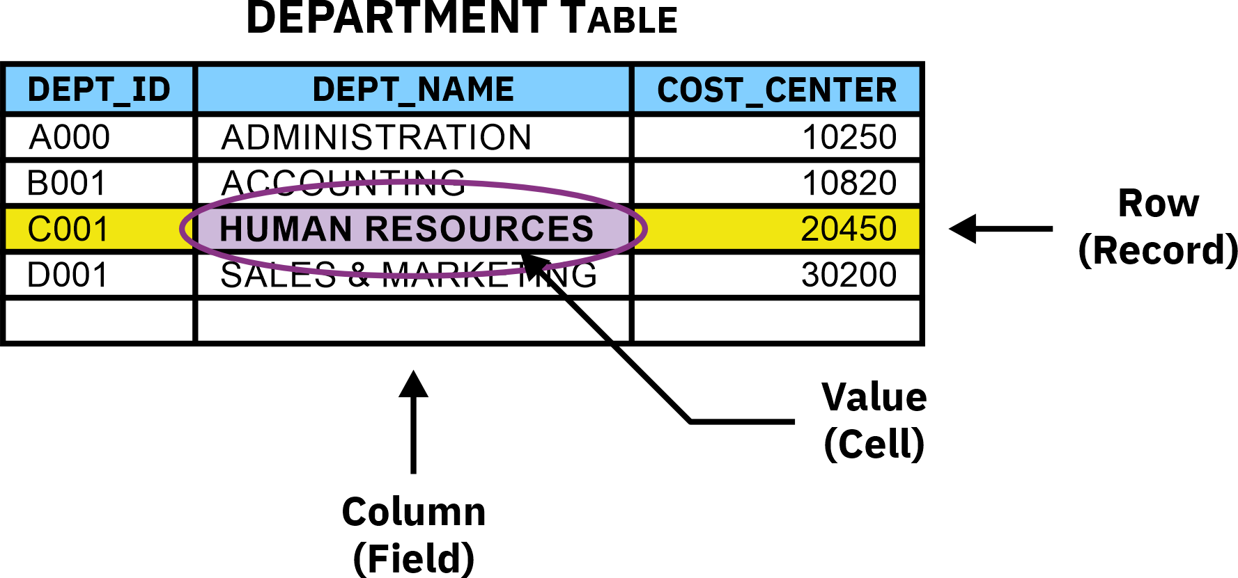
Figure 1: Structure of a table

Tables are created by executing the CREATE TABLE SQL statement. In its simplest form, the syntax for this statement looks like this:

CREATE TABLE [ TableName ] ( [ Element ] , ... )
< ORGANIZE BY [ ROW | COLUMN ] >

where:

•	TableName	:	Identifies the name to assign to the table that is to be created.
•	Element	:	Identifies one or more columns, UNIQUE constraints, CHECK constraints, referential constraints, informational constraints, and/or a primary key constraint to include in the table definition.

The syntax used to define each element varies according to the element specified — the basic syntax used to define a column element (which is the most common type of element used) is:

[ ColumnName ] [ DataType ]
< NOT NULL >
< WITH DEFAULT < [ DefaultValue ] | NULL > >
< UniqueConstraint >
< CheckConstraint >
< RIConstraint >

where:

•	ColumnName	:	Identifies the name to assign to the column; the name specified must be unique.
•	DataType	:	Identifies the data type to assign to the column; the data type determines the kind of data values that can be stored in the column. (You can learn more about the data types available with Db2 here: Data types)
•	DefaultValue	:	Identifies the default value to provide for the column if no value for the column is supplied when a new record is added to the table.
•	UniqueConstraint	:	Identifies a UNIQUE or primary key constraint that is to be associated with the column. A UNIQUE constraint can be used to ensure that values assigned to one or more columns of a table are never duplicated; a primary key is a special form of a UNIQUE constraint that uniquely defines the characteristics of each table row. (You can learn more about UNIQUE and primary key constraints here: Types of constraints)
•	CheckConstraint	:	Identifies a CHECK constraint that is to be associated with the column. A CHECK constraint can be used to ensure that a particular column in a table is never assigned an unacceptable value. (You can learn more about check constraints here: Types of constraints)
•	RIConstraint	:	Identifies a referential integrity constraint that is to be associated with the column. Referential integrity constraints (also known as referential constraints and foreign key constraints) can be used to define required relationships between select columns and tables. (You can learn more about referential integrity constraints here: Types of constraints)

Therefore, to create a table named EMPLOYEES that contains three columns, one of which is named EMPID that will be used to store integer data, one that is named NAME that can contain up to 30 characters, and one that is named DEPT that will be used to store fixed-length character string data that is three characters long, you would execute a CREATE TABLE statement that looks like this:

CREATE TABLE employees (empid INTEGER, name VARCHAR(30), dept CHAR(3))

Execute the code:

The code in the next cell builds a CREATE TABLE statement and then executes it to create a table named EMPLOYEE. (This table will be used by other exercises in this lab.) It then queries the system catalog to verify that the EMPLOYEE table exists.

Select the code cell below and carefully read through the comments. This will help you understand the actions the code performs.

When you are ready, click on the

button or press Shift+Enter to execute the code.

In [ ]:

#----------------------------------------------------------------------------------------------#
# Create A Table Named EMPLOYEE In The Database                                                #
#----------------------------------------------------------------------------------------------#

# Define And Initialize The Appropriate Variables
sqlStatement = ""                               # Structured Query Language (SQL) Statement
resultSet = False                               # Pointer To A Result Set
errorMsg = ""                                   # Detailed Error Information
columnHeaders = ("TABLE_NAME", "NUM_COLUMNS")   # Result Set Column Headers Tuple
columnWidths = (12, 11)                         # Result Set Column Widths Tuple
retCode = True                                  # Return Code

# Define The CREATE TABLE Statement To Be Executed
sqlStatement = "CREATE TABLE employee ("  # Create A Table Named EMPLOYEE
sqlStatement += " empno INTEGER,"         # With A Column Named EMPNO That Accepts Integers
sqlStatement += " name VARCHAR(30),"      # And A Column Named NAME That Accepts 30 Characters
sqlStatement += " hiredate DATE,"         # And A Column Named HIREDATE That Accepts Dates
sqlStatement += " title CHAR(25),"        # And A Column Named TITLE That Accepts 25 Characters
sqlStatement += " dept CHAR(3),"          # And A Column Named DEPT That Accepts 3 Characters
sqlStatement += " salary DECIMAL(8,2))"   # And A Column Named SALARY That Accepts Numbers
                                          #   With A Total Of 8 Digits And 2 Decimal Places

# Execute The CREATE TABLE Statement Just Defined By Calling The ibm_db.exec_immediate() API
# (This API Prepares And Executes An SQL Statement In A Single Step)
print("\nExecuting the following SQL statement:\n\n" + sqlStatement)
try:
    resultSet = ibm_db.exec_immediate(connectionID, sqlStatement)
except Exception:
    print("\nERROR: Unable to execute the SQL statement specified.\n")    
    pass

# If The SQL Statement Could Not Be Executed, Display A Detailed Error Message And Exit
# (Call The ibm_db.stmt_errormsg() API To Obtain Detailed Error Information)
if resultSet == False:
    errorMsg = ibm_db.stmt_errormsg()
    print(errorMsg + "\n")
    exit(-1)
    
# Otherwise, Print "Done" And Display A Section Divider Line
else:
    print("\nDone!\n")
    print('*' * 100)
    
#----------------------------------------------------------------------------------------------#
# Retrieve Information About The EMPLOYEE Table From The System Catalog                        #
#----------------------------------------------------------------------------------------------#

# Define The SQL Statement To Be Executed
sqlStatement = "SELECT TABNAME, COLCOUNT"       # Retreive The Data Stored In These Columns
sqlStatement += " FROM SYSCAT.TABLES"           # From The SYSCAT.TABLES View
sqlStatement += " WHERE TABNAME = 'EMPLOYEE'"   # For A Table Named 'EMPLOYEE'

# Execute The SQL Statement Just Defined By Calling The runQuery() Function Defined Earlier
# (Pass It The SQL Statement To Be Executed, Along With The Tuples That Contain Column Header
# And Column Width Information)
retCode = runQuery(0, sqlStatement, columnHeaders, columnWidths)

# If The SQL Statement Was Successfully Executed, Add A Blank Line To The End Of The Report
if retCode == True:
    print()

Step 4: Insert a record into the EMPLOYEE table

Overview:

When a table is first created, it is nothing more than a definition of how a set of data values are to be stored — no data is actually stored in it. But once created, a table can be populated in a variety of ways. For example, it can be bulk-loaded using Db2 utilities like Import, Ingest, and Load. Or, data can be added to it, one record (row) at a time, using the INSERT SQL statement.

The basic syntax for the INSERT statement looks like this:

INSERT INTO [ TableName | ViewName ]
< ( [ ColumnName ] , ... ) >
VALUES ( [ Value | NULL | DEFAULT ] , ... )

where:

•	TableName	:	Identifies, by name, the table data is to be added to; this can be any type of table except a system catalog table or a system-maintained materialized query table (MQT).
•	ViewName	:	Identifies, by name, the view data is to be added to; this can be any type of view except a system catalog view or a read-only view.
•	ColumnName	:	Identifies, by name, one or more columns that data values are to be assigned to; each column name provided must identify an existing column in the table or view specified.
•	Value	:	Identifies one or more data values that are to be added to the table or view specified.

Thus, to add a record to a table named DEPARTMENT that was created using a CREATE TABLE statement that looked like this:

CREATE TABLE department (deptno CHAR(3), deptname CHAR(20), mgrid INTEGER)

You might execute an INSERT statement that looks like this:

INSERT INTO department (deptno, deptname, mgrid) VALUES ('A01', 'ADMINISTRATION', 1000)

It is important to note that the number of values provided in the VALUES clause must equal the number of column names identified in the column name list. The values provided will be assigned to columns in the order in which they appear — in other words, the first value listed will be assigned to the first column identified, the second value will be assigned to the second column identified, and so on. In addition, each value supplied must be compatible with the data type of the column it is being assigned to. (For example, a character string value can only be assigned to a column that has character string data type.)

If values are provided for every column found in the table, the column name list can be omitted. In this case, the first value provided is assigned to the first column in the table, the second value is assigned to the second column, and so on. Thus, the record that was added to the DEPARTMENT table in the previous example could just as easily have been added by executing an INSERT statement that looks like this:

INSERT INTO department VALUES ('A01', 'ADMINISTRATION', 1000)

Along with literal values, two special tokens can also be used to assign values to individual columns. The first token, DEFAULT, is used to assign a system- or user-supplied value to a column that was defined as having a default constraint when the table was created. The second, the NULL token, is used to assign a NULL value to any nullable column — that is, any column that was not defined as having a NOT NULL constraint.

Therefore, you could add a record that contains a NULL value for the MGRID column to the DEPARTMENT table defined earlier by executing an INSERT statement that looks like this:

INSERT INTO department VALUES ('A01', 'ADMINISTRATION', NULL)

Execute the code:

The code in the next cell drops (removes) the table named EMPLOYEE that was created earlier.

Select the code cell below and carefully read through the comments. This will help you understand the actions the code performs.

When you are ready, click on the

button or press Shift+Enter to execute the code.

In [ ]:

#----------------------------------------------------------------------------------------------#
# Insert A Record Into The EMPLOYEE Table Created Earlier                                      #
#----------------------------------------------------------------------------------------------#

# Define And Initialize The Appropriate Variables
sqlStatement = ""                               # Structured Query Language (SQL) Statement
resultSet = False                               # Pointer To A Result Set
errorMsg = ""                                   # Detailed Error Information
retCode = True                                  # Return Code

# Define The INSERT Statement That Is To Be Used To Add Data To The EMPLOYEE Table
sqlStatement = "INSERT INTO employee"    # Insert Into The EMPLOYEE Table
sqlStatement += " VALUES(1000,"          # The Value 1000 For The EMPNO Column
sqlStatement += " 'JAMES DEAN',"         # The Value 'JAMES DEAN' For The NAME Column
sqlStatement += " '04/20/2010',"         # The Value '04/20/2010 For The HIREDATE Column
sqlStatement += " 'PRESIDENT',"          # The Value 'PRESIDENT' For The TITLE Column
sqlStatement += " 'A01',"                # The Value 'A01' For The DEPT Column
sqlStatement += " 158096.00)"            # And The Value 158096.00 For The SALARY Column

# Execute The SQL Statement Just Defined By Calling The ibm_db.exec_immediate() API
# (This API Prepares And Executes An SQL Statement In A Single Step)
print("\nExecuting the following SQL statement:\n\n" + sqlStatement)
try:
    resultSet = ibm_db.exec_immediate(connectionID, sqlStatement)
except Exception:
    print("\nERROR: Unable to execute the SQL statement specified.\n")    
    pass

# If The SQL Statement Could Not Be Executed, Display A Detailed Error Message And Exit
# (Call The ibm_db.stmt_errormsg() API To Obtain Detailed Error Information)
if resultSet == False:
    errorMsg = ibm_db.stmt_errormsg()
    print(errorMsg + "\n")
    exit(-1)

# Otherwise, Print "Done" And Display A Section Divider Line
else:
    print("\nDone!\n")
    print('*' * 100)
    
#----------------------------------------------------------------------------------------------#
# Query The EMPLOYEE Table To Verify The Data Was Added                                        #
#----------------------------------------------------------------------------------------------#

# Define The SELECT Statement That Is To Be Executed
sqlStatement = "SELECT * FROM employee"        # Retreive All Data From The EMPLOYEE Table

# Define And Initialize A Column Headers Tuple 
columnHeaders = ("EMPNO", "NAME", "HIREDATE", "TITLE", "DEPT", "SALARY")

# Define And Initialize A Column Widths Tuple 
columnWidths = (5, 18, 10, 15, 4, 10)

# Execute The SQL Statement Just Defined By Calling The runQuery() Function Defined Earlier
# (Pass It The SQL Statement To Be Executed, Along With The Tuples That Contain Column Header
# And Column Width Information)
retCode = runQuery(0, sqlStatement, columnHeaders, columnWidths)

# If The SQL Statement Was Successfully Executed, Add A Blank Line To The End Of The Report
if retCode == True:
    print()

Step 5: Add additional records to the EMPLOYEE table using a prepared INSERT statement with parameter markers

Overview:

With Python and Jupyter Notebook (as well as many other programming languages), there are two ways in which SQL statements can be executed:

Prepare and then execute: This approach separates the preparation of an SQL statement from its actual execution and is typically used when a statement is to be executed repeatedly (often with different values being supplied for place holders in the statement with each execution). This method is also used when an application needs to know information about the columns that will exist in the result set produced by the statement, in advance. The ibm_db.prepare( ) and ibm_db.execute( ) application programming interfaces (APIs) in the ibm_db library are used to process SQL statements in this manner.
Execute immediately: This approach combines the preparation and execution of an SQL statement into a single step and is typically used when a statement only needs to be executed once. The ibm_db.exec_immediate( ) API in the ibm_db library is used to process SQL statements in this manner. (This has been the approach used in the lab exercises thus far.)

Both methodologies allow the use of parameter markers in place of constants or expressions in the SQL statements used; however, parameter markers are typically not used if the statement is only going to be executed once. Parameter markers are represented by question mark (?) characters and indicate positions in an SQL statement where the value of one or more variables is to be substituted at the time the statement is executed. If an application variable is associated with a specific parameter marker in an SQL statement, that variable is said to be “bound” to the parameter marker and such bindings can be made by executing the ibm_db.bind_param( ) API. That said, with Python and Jupyter Notebook, application variables do not have to be explicitly bound in order to be used to provide values to parameter markers during SQL statement execution — values can be passed, via a Python tuple, when the ibm_db.execute( ) or ibm_db.exec_immediate( ) API is called. However, binding gives you more control over the parameter type (input, output, or input/output), SQL data type, precision, and scale that are used for the parameter marker values provided. (To keep things simple, Python tuples will be used to provide values for parameter markers used throughout this lab.)

Execute the code:

The code in the next cell builds an INSERT statement with parameter markers, prepares it, and then executes it repeatedly to add several different records to the EMPLOYEE table created earlier. It then queries the table to verify the records were successfully added.

Select the code cell below and carefully read through the comments. This will help you understand the actions the code performs.

When you are ready, click on the

button or press Shift+Enter to execute the code.

In [ ]:

#----------------------------------------------------------------------------------------------#
# Populate The EMPLOYEE Table Using A Prepared INSERT Statement With Parameter Markers         #
#----------------------------------------------------------------------------------------------#

# Define And Initialize The Appropriate Variables
sqlStatement = ""                               # Structured Query Language (SQL) Statement
preparedStmt = None                             # Pointer To A Prepared SQL Statement
errorMsg = ""                                   # Detailed Error Information
recIndex = 0                                    # Records List Index
retCode = True                                  # Return Code

# Define The INSERT Statement To Be Used To Add Data To The EMPLOYEE Table
sqlStatement = "INSERT INTO employee"    # Insert Into The EMPLOYEE Table
sqlStatement += " VALUES(?,"             # The Parameter Marker For The EMPNO Column Value
sqlStatement += " ?,"                    # The Parameter Marker For The NAME Column Value
sqlStatement += " ?,"                    # The Parameter Marker For The HIREDATE Column Value
sqlStatement += " ?,"                    # The Parameter Marker For The TITLE Column Value
sqlStatement += " ?,"                    # The Parameter Marker For The DEPT Column Value
sqlStatement += " ?)"                    # And The Parameter Marker For The SALARY Column Value

# Prepare The INSERT Statement Just Defined By Calling The ibm_db.prepare() API
print("\nPreparing the following SQL statement for repetitive execution:\n\n" + sqlStatement)
try:
    preparedStmt = ibm_db.prepare(connectionID, sqlStatement)
except Exception:
    print("\nERROR: Unable to prepare the SQL statement specified.\n")
    pass

# If The SQL Statement Could Not Be Prepared, Display A Detailed Error Message And Exit
# (Call The ibm_db.stmt_errormsg() API To Obtain Detailed Error Information)
if preparedStmt == None:
    errorMsg = ibm_db.stmt_errormsg()
    print(errorMsg + "\n")
    exit(-1)
    
# Otherwise, Print "Done" And Display A Section Divider Line
else:
    print("\nDone!\n")
    print('*' * 100)
    print()

#----------------------------------------------------------------------------------------------#
# Generate The Data                                                                            #
#----------------------------------------------------------------------------------------------#

# Define And Initialize An EMPNO Column Values List
empNo = [1001, 1002, 1003, 1004, 1005, 1006, 1007, 1008, 1009]

# Define And Initialize A NAME Column Values List
empName = ['MARILYN MONROE', 'HUMPHREY BOGART', 'INGRID BERGMAN', 'JAMES CAGNEY']
empName += ['WILLIAM HOLDEN', 'JACK LEMMON', 'WALTER MATTHAU', 'KATHARINE HEPBURN']
empName += ['AVA GARDNER']

# Define And Initialize A HIREDATE Column Values List
hireDate = ['05/10/2014', '09/15/2012', '02/14/2011', '10/31/2012', '01/02/2020']
hireDate += ['07/04/2010', '10/12/2018', '03/15/2016', '06/06/2017']

# Define And Initialize A TITLE Column Values List
empTitle = ['ENGINEER', 'ANALYST', 'PROGRAMMER', 'TECHNICIAN', 'MANAGER']
empTitle += ['ANALYST', 'PROGRAMMER', 'MANAGER', 'TECHNICIAN']

# Define And Initialize A DEPT Column Values List
deptNo = ['B01', 'C01', 'C01', 'E01', 'F01', 'E01', 'D01', 'F01', 'B01']

# Define And Initialize A SALARY Column Values List
empSalary = [103675.00, 88192.00, 99475.50, 105787.00, 85428.50, 112515.00]
empSalary += [106943.50, 129081.50, 118903.00]

# Create A List Of Data Record Tuples, Using The Column Value Lists Just Defined
dataRecords = list(zip(empNo, empName, hireDate, empTitle, deptNo, empSalary))

# Display A Message Stating The Prepared Statement Is Being Executed
print("Executing the prepared SQL statement ... ", end="")

#----------------------------------------------------------------------------------------------#
# Populate The Table                                                                           #
#----------------------------------------------------------------------------------------------#

# As Long As There Are Data Record Tuples Available, ...
while recIndex < len(dataRecords):
  
    # Execute The INSERT Statement Prepared Earlier By Calling The ibm_db.execute() API
    # (Provide The Current Data Record Tuple As An Input Value)
    try:
        retCode = ibm_db.execute(preparedStmt, dataRecords[recIndex])
    except Exception:
        print("\nERROR: Unable to execute the prepared INSERT statement.\n")    
        pass
    
    # If The Prepared INSERT Statement Could Not Be Executed, Display A Detailed Error
    # Message And Exit (Call The ibm_db.stmt_errormsg() API To Obtain Detailed Error
    # Information)
    if retCode == False:
        errorMsg = ibm_db.stmt_errormsg()
        print(errorMsg + "\n")
        exit(-1)   

    # Otherwise, Increment The Record Index
    else:
        recIndex = recIndex + 1
    
# Print "Done" And Display Another Section Divider Line
print("Done!\n")
print('*' * 100)
print()

#----------------------------------------------------------------------------------------------#
# Query The Table To Verify The Data Was Added                                                 #
#----------------------------------------------------------------------------------------------#

# Define The SELECT Statement That Is To Be Executed
sqlStatement = "SELECT * FROM employee"        # Retreive All Data From The EMPLOYEE Table

# Initialize The Result Set Column Headers And Column Widths Tuples
columnHeaders = ("EMPNO", "NAME", "HIREDATE", "TITLE", "DEPT", "SALARY")
columnWidths = (5, 18, 10, 15, 4, 10)

# Display A Header For The Query Results That Are About To Be Displayed 
print("Data stored in the EMPLOYEE table:")

# Execute The SQL Statement Just Defined By Calling The runQuery() Function Defined Earlier
# (Pass It The SQL Statement To Be Executed, Along With The Tuples That Contain Column Header
# And Column Width Information)
retCode = runQuery(1, sqlStatement, columnHeaders, columnWidths)

# If The SQL Statement Was Successfully Executed, Add A Blank Line To The End Of The Report
if retCode == True:
    print()

Step 6: Create a second table named DEPARTMENT and populate it

Overview:

The next exercise uses both the EMPLOYEE table that was just populated and a second table named DEPARTMENT. Therefore, a table named DEPARTMENT needs to be created and populated.

Execute the code:

The code in the next cell creates a table named DEPARTMENT and uses an INSERT statement with parameter markers to populate it. It then queries the table to verify the table exists and that 6 records have been added to it.

Select the code cell below and carefully read through the comments. This will help you understand the actions the code performs.

When you are ready, click on the

button or press Shift+Enter to execute the code.

In [ ]:

#----------------------------------------------------------------------------------------------#
# Create A Table Named DEPARTMENT In The Database                                              #
#----------------------------------------------------------------------------------------------#

# Define And Initialize The Appropriate Variables
sqlStatement = ""                               # Structured Query Language (SQL) Statement
resultSet = False                               # Pointer To A Result Set
errorMsg = ""                                   # Detailed Error Information
preparedStmt = None                             # Pointer To A Prepared SQL Statement
recIndex = 0                                    # Records List Index
retCode = True                                  # Return Code

# Define The CREATE TABLE Statement To Be Executed
sqlStatement = "CREATE TABLE department (" # Create A Table Named DEPARTMENT
sqlStatement += "code CHAR(3), "           # With A Column Named CODE That Accepts 3 Characters
sqlStatement += "desc VARCHAR(30)) "       # And A Column Named DESC That Accepts 30 Characters

# Execute The CREATE TABLE Statement Just Defined By Calling The ibm_db.exec_immediate() API
# (This API Prepares And Executes An SQL Statement In A Single Step)
print("\nExecuting the following SQL statement:\n\n" + sqlStatement)
try:
    resultSet = ibm_db.exec_immediate(connectionID, sqlStatement)
except Exception:
    print("\nERROR: Unable to execute the SQL statement specified.\n")    
    pass

# If The SQL Statement Could Not Be Executed, Display A Detailed Error Message And Exit
# (Call The ibm_db.stmt_errormsg() API To Obtain Detailed Error Information)
if resultSet == False:
    errorMsg = ibm_db.stmt_errormsg()
    print(errorMsg + "\n")
    exit(-1)
    
# Otherwise, Print "Done" And Display A Section Divider Line
else:
    print("\nDone!\n")
    print('*' * 100)
    print()
    
#----------------------------------------------------------------------------------------------#
# Create And Prepare An INSERT Statement With Parameter Markers                                #
#----------------------------------------------------------------------------------------------#
    
# Define The INSERT Statement To Be Used To Add Data To The DEPARTMENT Table
sqlStatement = "INSERT INTO department"    # Insert Into The DEPARTMENT Table
sqlStatement += " VALUES(?,"               # The Parameter Marker For The CODE Column Value
sqlStatement += " ?)"                      # And The Parameter Marker For The DESC Column Value

# Prepare The INSERT Statement Just Defined By Calling The ibm_db.prepare() API
print("Preparing the following SQL statement for repetitive execution:\n\n" + sqlStatement)
try:
    preparedStmt = ibm_db.prepare(connectionID, sqlStatement)
except Exception:
    print("\nERROR: Unable to prepare the SQL statement specified.\n")
    pass

# If The SQL Statement Could Not Be Prepared, Display A Detailed Error Message And Exit
# (Call The ibm_db.stmt_errormsg() API To Obtain Detailed Error Information)
if preparedStmt == None:
    errorMsg = ibm_db.stmt_errormsg()
    print(errorMsg + "\n")
    exit(-1)
    
# Otherwise, Print "Done" And Display A Section Divider Line
else:
    print("\nDone!\n")
    print('*' * 100)
    print()
    
#----------------------------------------------------------------------------------------------#
# Generate The Data And Populate The Table                                                     #
#----------------------------------------------------------------------------------------------#    
    
# Define And Initialize An CODE Column Values List
deptCode = ['A01', 'B01', 'C01', 'D01', 'E01', 'F01']

# Define And Initialize A DESC Column Values List
deptDesc = ['ADMINISTRATION', 'PLANNING', 'DEVELOPMENT', 'PERSONNEL', 'OPERATIONS', 'SUPPORT']

# Create A List Of Data Record Tuples, Using The Column Value Lists Just Defined
dataRecords = list(zip(deptCode, deptDesc))

# Display A Message Stating The Prepared Statement Is Being Executed
print("Executing the prepared SQL statement ... ", end="")

# As Long As There Are Data Record Tuples Available, ...
while recIndex < len(dataRecords):

    # Execute The INSERT Statement Prepared Earlier By Calling The ibm_db.execute() API
    # (Provide The Current Data Record Tuple As An Input Value)
    try:
        retCode = ibm_db.execute(preparedStmt, dataRecords[recIndex])
    except Exception:
        print("\nERROR: Unable to execute the prepared INSERT statement.\n")    
        pass
    
    # If The Prepared INSERT Statement Could Not Be Executed, Display A Detailed Error
    # Message And Exit (Call The ibm_db.stmt_errormsg() API To Obtain Detailed Error
    # Information)
    if retCode == False:
        errorMsg = ibm_db.stmt_errormsg()
        print(errorMsg + "\n")
        exit(-1)   

    # Otherwise, Increment The Record Index
    else:
        recIndex = recIndex + 1
    
# Print "Done" And Display Another Section Divider Line
print("Done!\n")
print('*' * 100)
print()

#----------------------------------------------------------------------------------------------#
# Query The Table To Verify The Data Was Added                                                 #
#----------------------------------------------------------------------------------------------#

# Define The SELECT Statement That Is To Be Executed
sqlStatement = "SELECT * FROM department"        # Retreive All Data From The DEPARTMENT Table

# Initialize The Result Set Column Headers And Column Widths Tuples
columnHeaders = ("CODE", "DESC")
columnWidths = (4, 18)

# Display A Header For The Query Results That Are About To Be Displayed 
print("Data stored in the DEPARTMENT table:")

# Execute The SQL Statement Just Defined By Calling The runQuery() Function Defined Earlier
# (Pass It The SQL Statement To Be Executed, Along With The Tuples That Contain Column Header
# And Column Width Information)
retCode = runQuery(1, sqlStatement, columnHeaders, columnWidths)

# If The SQL Statement Was Successfully Executed, Add A Blank Line To The End Of The Report
if retCode == True:
    print()

Step 7: Create a view named EMP_DEPT

Overview:

A view is a database object that is used to provide an alternative way of describing and displaying data stored in one or more tables. As with tables, views can be thought of as having columns and rows; unlike tables, views do not contain data. Instead, a view is essentially a named specification of a result table that is populated whenever the view is referenced. (Each time a view is referenced, a query is executed, and the results are retrieved from one or more underlying tables and returned in a table-like format.) The following illustration shows how a simple view that presents data from two different tables might look:

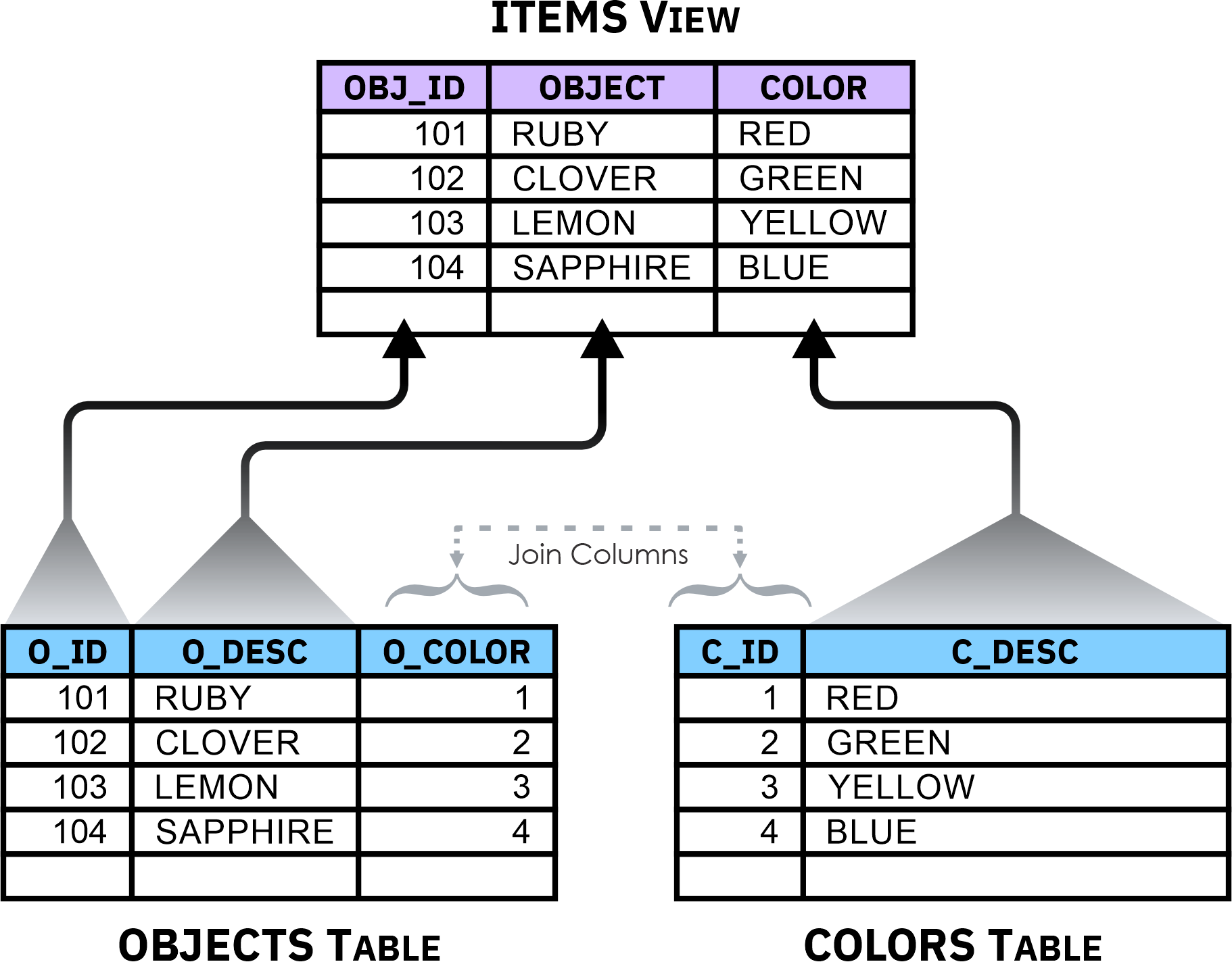
Figure 2: A view that presents data stored in two different tables

Because views look similar to tables, in most cases they can be referenced in the same way that tables can be referenced. That is, they can be the source of queries as well as the target of INSERT, UPDATE, and DELETE operations. (We will take a closer look at the UPDATE and DELETE statements shortly.) When a view is the target of such an operation, the query that was used to define the view is executed and the operation is performed on the results — the operation itself is actually executed against the base table(s) the view is derived from. (If a view is derived from other views, the operation cascades down through all applicable views until it reaches the appropriate table/tables.)

It is important to note that a single base table can serve as the source of multiple views; the SQL query provided as part of a view’s definition determines the data that is to be presented when the view is referenced. Because of this, views are sometimes used to control access to sensitive data. For example, if a table contains information about every employee who works for a company (including sensitive information like bank account numbers used for direct deposit), managers might access this table via a view that allows them to see only non-sensitive information about employees who report directly to them. Similarly, Human Resources personnel could be given access to the table by means of a view that lets them see only the information needed to generate employee paychecks. Because each set of users are given access to data through different views, they each see different presentations of data that resides in the same table.

Views are created by executing the CREATE VIEW SQL statement. In its simplest form, the syntax for this statement looks like this:

CREATE VIEW [ ViewName ]
< ( [ ColumnName ] , ... ) >
AS [ SELECTStmnt ]

where:

•	ViewName	:	Identifies the name to assign to the view that is to be created.
•	ColumnName	:	Identifies, by name, one or more columns that are to be included in the view — if a list of column names is provided, the number of column names supplied must match the number of columns that will be returned by the SELECT statement used to create the view; otherwise, if a list of column names is not provided, the view will inherit the names assigned to the columns returned by the SELECT statement used.
•	SELECTStmnt	:	Identifies a SELECT statement that, when executed, will produce the data values that are to be used to populate the view (by retrieving them from other tables and/or views).

Therefore, to create a view named LARGE_DEPTS that references three specific columns found in a table named DEPARTMENT, you might execute a CREATE VIEW statement that looks something like this:

CREATE VIEW large_depts AS SELECT (dept_no, dept_name, dept_size) FROM department WHERE dept_size > 25

The resulting view will contain department number (DEPT_NO), department name (DEPT_NAME), and department size (DEPT_SIZE) information for every department that has more than 25 people assigned to it.

Execute the code:

The code in the next cell builds a CREATE VIEW statement that references the EMPLOYEE and DEPARTMENT tables created earlier. It then executes the statement to create a view named EMP_DEPT. Next, it queries the system catalog to verify that the EMP_DEPT view exists. Finally, it executes a query that uses the EMP_DEPT view as a data source and displays the records retrieved.

Select the code cell below and carefully read through the comments. This will help you understand the actions the code performs.

When you are ready, click on the

button or press Shift+Enter to execute the code.

In [ ]:

#----------------------------------------------------------------------------------------------#
# Create A View Named EMP_DEPT In The Database                                                 #
#----------------------------------------------------------------------------------------------#

# Define And Initialize The Appropriate Variables
sqlStatement = ""                               # Structured Query Language (SQL) Statement
resultSet = False                               # Pointer To A Result Set
errorMsg = ""                                   # Detailed Error Information
recIndex = 0                                    # Records List Index
retCode = True                                  # Return Code

# Define The CREATE VIEW Statement To Be Executed
sqlStatement = "CREATE VIEW emp_dept"           # Create A View Named EMP_DEPT
sqlStatement += " (empno,"                      # That Has A Column Named EMPNO
sqlStatement += " name,"                        # And A Column Named NAME
sqlStatement += " department)"                  # And A Column Named DEPARTMENT
sqlStatement += " AS SELECT"                    # Using A SELECT Statement
sqlStatement += " e.empno,"                     # That Retreives Data From The EMPNO Column
sqlStatement += " e.name,"                      # And The NAME Column
sqlStatement += " d.desc"                       # And The DESCRIPTION Column
sqlStatement += " FROM employee AS e,"          # Found In The EMPLOYEE Table (Referenced As E)
sqlStatement += " DEPARTMENT AS d"              # And The DEPARTMENT Table (Referenced As D)
sqlStatement += " WHERE e.dept = d.code"        # Where Values In The DEPT Column Of The EMPLOYEE
                                                #   Table Match The Values Of The CODE Column Of
                                                #   The DEPARTMENT Table

# Execute The CREATE VIEW Statement Just Defined By Calling The ibm_db.exec_immediate() API
# (This API Prepares And Executes An SQL Statement In A Single Step)
print("\nExecuting the following SQL statement:\n\n" + sqlStatement)
try:
    resultSet = ibm_db.exec_immediate(connectionID, sqlStatement)
except Exception:
    print("\nERROR: Unable to execute the SQL statement specified.\n")    
    pass

# If The SQL Statement Could Not Be Executed, Display A Detailed Error Message And Exit
# (Call The ibm_db.stmt_errormsg() API To Obtain Detailed Error Information)
if resultSet == False:
    errorMsg = ibm_db.stmt_errormsg()
    print(errorMsg + "\n")
    exit(-1)
    
# Otherwise, Print "Done" And Display A Section Divider Line
else:
    print("\nDone!\n")
    print('*' * 100)
      
#----------------------------------------------------------------------------------------------#
# Retrieve Information About The EMP_DEPT View From The System Catalog                         #
#----------------------------------------------------------------------------------------------#

# Initialize The Result Set Column Headers And Column Widths Tuples
columnHeaders = ("TABLE_NAME", "NUM_COLUMNS")
columnWidths = (12, 11)

# Define The SQL Statement To Be Executed
sqlStatement = "SELECT TABNAME, COLCOUNT"       # Retreive The Data Stored In These Columns
sqlStatement += " FROM SYSCAT.TABLES"           # From The SYSCAT.TABLES View
sqlStatement += " WHERE TYPE = 'V'"             # Where The TYPE Column Value Indicates VIEW
sqlStatement += " AND TABSCHEMA"                # And The Schema Name
sqlStatement += " NOT LIKE 'SYS%'"              # Does NOT Start With 'SYS'

# Execute The SQL Statement Just Defined By Calling The runQuery() Function Defined Earlier
# (Pass It The SQL Statement To Be Executed, Along With The Tuples That Contain Column Header
# And Column Width Information)
retCode = runQuery(0, sqlStatement, columnHeaders, columnWidths)

# If The SQL Statement Was Successfully Executed, Print A Blank Line And Display Another
# Section Divider Line
if retCode == True:
    print()
    print('*' * 100)

#----------------------------------------------------------------------------------------------#
# Query The EMP_DEPTS View To See Its Records                                                  #
#----------------------------------------------------------------------------------------------#

# Define The SQL Statement That Is To Be Executed
sqlStatement = "SELECT * FROM emp_dept"    # Retreive All Data From The EMP_DEPT View

# Initialize The Result Set Column Headers And Column Widths Tuples
columnHeaders = ("EMPNO", "NAME", "DEPARTMENT")
columnWidths = (6, 18, 20)

# Execute The SQL Statement Just Defined By Calling The runQuery() Function Defined Earlier
# (Pass It The SQL Statement To Be Executed, Along With The Tuples That Contain Column Header
# And Column Width Information)
retCode = runQuery(0, sqlStatement, columnHeaders, columnWidths)

# If The SQL Statement Was Successfully Executed, Add A Blank Line To The End Of The Report
if retCode == True:
    print()

Step 8: Change a record in the EMPLOYEE table

Overview:

Data in a database is rarely static. Over time, the need to change or remove one or more values stored in a table can, and will, arise. This is where the UPDATE statement comes into play — once a table has been created and populated, any of the data values stored in it can be modified by executing this statement. The basic syntax for the UPDATE statement is:

UPDATE [ TableName | ViewName]
SET [ ColumnName ] = [ Value | NULL | DEFAULT] , ... ]
< WHERE [Condition] >

UPDATE [ TableName | ViewName ]
SET ( [ColumnName] , ... ) =
( [Value | NULL | DEFAULT] , ... )
< WHERE [ Condition ] >

where:

•	TableName	:	Identifies, by name, the table that contains the data that is to be modified; this can be any type of table except a system catalog table or a system-maintained materialized query table (MQT).
•	ViewName	:	Identifies, by name, the view data that contains the data that is to be modified; this can be any type of view except a system catalog view or a read-only view.
•	ColumnName	:	Identifies, by name, one or more columns that contain data that is to be modified; each column name provided must identify an existing column in the table or view specified.
•	Value	:	Identifies one or more data values that are to be used to replace existing values for the *ColumnName*(s) specified.
•	Condition	:	Identifies the search criterion, in the form of a WHERE clause, that is to be used to locate one or more specific rows whose data values are to be modified.

NOTE: In most cases, an appropriate WHERE clause and Condition should be provided with an UPDATE statement. Otherwise, the update operation specified will be performed against every record in the table or view referenced.

Thus, to change the records stored in the EMPLOYEE table created earlier such that the SALARY of every employee with the title of ANALYST is increased by 6%, you would execute an UPDATE statement that looks like this:

UPDATE employee SET salary = salary * 1.06 WHERE title = 'ANALYST'

In addition to providing a way to change existing data values, the UPDATE statement can also be used to remove data stored in one or more columns that are nullable (by changing the existing data value to NULL). For example, to delete the values assigned to the DEPT column of every record found in the EMPLOYEE table created earlier, you could execute an UPDATE statement that looks like this:

UPDATE employee SET dept = NULL

NOTE: Unlike other database management systems, Db2 is intelligent enough to know whether an UPDATE operation actually changes a record's data. If an UPDATE statement is executed, but no changes are actually made, Db2 will not log the operation or attempt to write the record to disk. In fact, it's possible to determine just how many unchanged UPDATE operations have been performed against a table by examining the NO_CHANGE_UPDATES information provided by the MON_GET_TABLE( ) monitoring function.

Execute the code:

The code in the next cell retrieves and displays a record from the EMPLOYEE table created earlier, modifies the record by executing an UPDATE statement, and then retrieves and displays the record again to verify that the changes desired were made.

Select the code cell below and carefully read through the comments. This will help you understand the actions the code performs.

When you are ready, click on the

button or press Shift+Enter to execute the code.

In [ ]:

#----------------------------------------------------------------------------------------------#
# Update A Record That Was Added To The EMPLOYEE Table Created Earlier                         #
#----------------------------------------------------------------------------------------------#

# Define And Initialize The Appropriate Variables
sqlStatement = ""                               # Structured Query Language (SQL) Statement
resultSet = False                               # Pointer To A Result Set
errorMsg = ""                                   # Detailed Error Information
retCode = True                                  # Return Code

#----------------------------------------------------------------------------------------------#
# Query The EMPLOYEE Table To See What A Specific Record Looks Like Before It Is Updated       #
#----------------------------------------------------------------------------------------------#

# Display A Message Indicating The "Before Update" Record Values Are Being Displayed
print("\nRECORD BEFORE THE UPDATE OPERATION")
print()

# Define The SQL Statement That Is To Be Executed
sqlStatement = "SELECT * FROM employee"    # Retreive All Data From The EMPLOYEE Table
sqlStatement += " WHERE empno = 1008"      # For The Record With An EMPNO Value Of 1008

# Initialize The Result Set Column Headers And Column Widths Tuples
columnHeaders = ("EMPNO", "NAME", "HIREDATE", "TITLE", "DEPT", "SALARY")
columnWidths = (5, 18, 10, 15, 4, 10)

# Execute The SQL Statement Just Defined By Calling The runQuery() Function Defined Earlier
# (Pass It The SQL Statement To Be Executed, Along With The Tuples That Contain Column Header
# And Column Width Information)
retCode = runQuery(2, sqlStatement, columnHeaders, columnWidths)

# If The SQL Statement Was Successfully Executed, Add A Blank Line To The End Of The Report
if retCode == True:
    print() 
    
# Display A Section Divider Line
print('*' * 100)
print()

#----------------------------------------------------------------------------------------------#
# Update A Record In The EMPLOYEE Table                                                        #
#----------------------------------------------------------------------------------------------#

# Define The UPDATE Statement That Will Be Used To Modify A Record In The EMPLOYEE Table
sqlStatement = "UPDATE employee"           # Change A Record In The EMPLOYEE Table
sqlStatement += " SET"                     # As Specified:
sqlStatement += " title = 'SR. MANAGER',"  # Change The TITLE Column Value To 'SR. MANAGER'
sqlStatement += " salary = salary * 1.10"  # And Raise The SALARY Column Value By 10%
sqlStatement += " WHERE empno = 1008"      # For The Employee With The EMPNO Value Of 1008

# Execute The SQL Statement Just Defined By Calling The ibm_db.exec_immediate() API
# (This API Prepares And Executes An SQL Statement In A Single Step)
print("Executing the following SQL statement:\n\n" + sqlStatement)
try:
    resultSet = ibm_db.exec_immediate(connectionID, sqlStatement)
except Exception:
    print("\nERROR: Unable to execute the SQL statement specified.\n")    
    pass

# If The SQL Statement Could Not Be Executed, Display A Detailed Error Message And Exit
# (Call The ibm_db.stmt_errormsg() API To Obtain Detailed Error Information)
if resultSet == False:
    errorMsg = ibm_db.stmt_errormsg()
    print(errorMsg + "\n")
    exit(-1)

# Otherwise, Print "Done" And Display A Section Divider Line
else:
    print("\nDone!\n")
    print('*' * 100)
    print()
    
#----------------------------------------------------------------------------------------------#
# Query The EMPLOYEE Table Again To Verify The Appropriate Updates Were Made                   #
#----------------------------------------------------------------------------------------------#

# Display A Message Indicating The "After Update" Record Values Are Being Displayed
print("RECORD AFTER THE UPDATE OPERATION")
print()

# Define The SQL Statement That Is To Be Executed
sqlStatement = "SELECT * FROM employee"    # Retreive All Data From The EMPLOYEE Table
sqlStatement += " WHERE empno = 1008"      # For The Record With The EMPNO Value Of 1008

# Execute The SQL Statement Just Defined By Calling The runQuery() Function Defined Earlier
# (Pass It The SQL Statement To Be Executed, Along With The Tuples That Contain Column Header
# And Column Width Information)
retCode = runQuery(2, sqlStatement, columnHeaders, columnWidths)

# If The SQL Statement Was Successfully Executed, Add A Blank Line To The End Of The Report
if retCode == True:
    print()

Step 9: Remove records from the EMPLOYEE table

Overview:

While the UPDATE statement can be used to remove values from individual columns (by replacing those values with NULL), it cannot be used to remove records. To remove one or more records from a table or view, the DELETE statement must be used instead. The basic syntax for this statement is:

DELETE FROM [ TableName | ViewName ]
< WHERE [ Condition ] >

where:

•	TableName	:	Identifies, by name, the table that contains the data that is to be deleted; this can be any type of table except a system catalog table or a system-maintained materialized query table (MQT).
•	ViewName	:	Identifies, by name, the view data that contains the data that is to be deleted; this can be any type of view except a system catalog view or a read-only view.
•	Condition	:	Identifies the search criterion, in the form of a WHERE clause, that is to be used to locate one or more specific rows whose data values are to be deleted.

NOTE: In most cases, an appropriate WHERE clause and Condition should be provided with a DELETE statement. Otherwise, every record stored in the table or view referenced will be removed (resulting in one or more empty tables).

Thus, to remove records stored in the EMPLOYEE table created earlier that are associated with employees who were hired before January 1, 2015, you would execute a DELETE statement that looks like this:

DELETE FROM employee WHERE hiredate < '12/31/2014'

Execute the code:

The code in the next cell retrieves and displays all of the records stored in the EMPLOYEE table created earlier, deletes some of these records by executing a DELETE statement, and then retrieves and displays the records again to verify the appropriate records were deleted.

Select the code cell below and carefully read through the comments. This will help you understand the actions the code performs.

When you are ready, click on the

button or press Shift+Enter to execute the code.

In [ ]:

#----------------------------------------------------------------------------------------------#
# Delete Records From The EMPLOYEE Table Created Earlier                                       #
#----------------------------------------------------------------------------------------------#

# Define And Initialize The Appropriate Variables
sqlStatement = ""                               # Structured Query Language (SQL) Statement
resultSet = False                               # Pointer To A Result Set
errorMsg = ""                                   # Detailed Error Information
retCode = True                                  # Return Code

#----------------------------------------------------------------------------------------------#
# Query The EMPLOYEE Table To See All OF The Records It Contains Before Some Are Deleted       #
#----------------------------------------------------------------------------------------------#

# Display A Message Indicating The "Before Update" Record Values Are Being Displayed
print("\nRECORDS BEFORE THE DELETE OPERATION")
print()

# Define The SQL Statement That Is To Be Executed
sqlStatement = "SELECT * FROM employee"    # Retreive All Data From The EMPLOYEE Table

# Initialize The Result Set Column Headers And Column Widths Tuples
columnHeaders = ("EMPNO", "NAME", "HIREDATE", "TITLE", "DEPT", "SALARY")
columnWidths = (5, 18, 12, 15, 4, 10)

# Execute The SQL Statement Just Defined By Calling The runQuery() Function Defined Earlier
# (Pass It The SQL Statement To Be Executed, Along With The Tuples That Contain Column Header
# And Column Width Information)
retCode = runQuery(1, sqlStatement, columnHeaders, columnWidths)

# If The SQL Statement Was Successfully Executed, Add A Blank Line To The End Of The Report
if retCode == True:
    print() 
    
# Display A Section Divider Line
print('*' * 100)
print()

#----------------------------------------------------------------------------------------------#
# Delete Select Records From The EMPLOYEE Table                                                #
#----------------------------------------------------------------------------------------------#

# Define The DELETE Statement That Will Be Used To Remove Records From The EMPLOYEE Table
sqlStatement = "DELETE FROM employee"       # Remove The Record From The EMPLOYEE Table
sqlStatement += " WHERE dept = 'E01'"       # For All Employees Who Are In Department E01

# Execute The SQL Statement Just Defined By Calling The ibm_db.exec_immediate() API
# (This API Prepares And Executes An SQL Statement In A Single Step)
print("Executing the following SQL statement:\n\n" + sqlStatement)
try:
    resultSet = ibm_db.exec_immediate(connectionID, sqlStatement)
except Exception:
    print("\nERROR: Unable to execute the SQL statement specified.\n")    
    pass

# If The SQL Statement Could Not Be Executed, Display A Detailed Error Message And Exit
# (Call The ibm_db.stmt_errormsg() API To Obtain Detailed Error Information)
if resultSet == False:
    errorMsg = ibm_db.stmt_errormsg()
    print(errorMsg + "\n")
    exit(-1)
    
# Otherwise, Print "Done" And Display A Section Divider Line
else:
    print("\nDone!\n")
    print('*' * 100)
    
#----------------------------------------------------------------------------------------------#
# Query The EMPLOYEE Table Again To Verify The Appropriate Records Were Deleted                #
#----------------------------------------------------------------------------------------------#

# Display A Message Indicating The "Before Update" Record Values Are Being Displayed
print("\nRECORDS AFTER THE DELETE OPERATION")
print()

# Define The SQL Statement That Is To Be Executed
sqlStatement = "SELECT * FROM employee"    # Retreive All Data From The EMPLOYEE Table

# Execute The SQL Statement Just Defined By Calling The runQuery() Function Defined Earlier
# (Pass It The SQL Statement To Be Executed, Along With The Tuples That Contain Column Header
# And Column Width Information)
retCode = runQuery(1, sqlStatement, columnHeaders, columnWidths)

# If The SQL Statement Was Successfully Executed, Add A Blank Line To The End Of The Report
if retCode == True:
    print()

Step 10: Create the tables that are used by the Db2 EXPLAIN facility

Overview:

When an SQL or XQuery statement is submitted to Db2 for processing, Db2's cost-based query optimizer analyzes it and generates several execution plans (known as access plans) that could potentially be used to perform the desired operation. It then estimates the execution cost of each plan and chooses the access plan that has the lowest anticipated cost.

If a static SQL or XQuery statement is embedded in an application, the optimal access plan is chosen at precompile time (or at bind time if deferred binding is used), and an executable form of this plan is stored in the system catalog as an object known as a package. If however, a dynamic statement is constructed at application run time (which is the case with all of the SQL statements used in this lab), access plans are generated when the statement is prepared for execution and the access plan chosen is stored in memory, temporarily (in what is known as the global package cache).

While Db2 provides several monitoring tools that can be used to obtain information about how well (or how poorly) some SQL operations perform, these tools cannot be used to examine the access plans that were chosen by the Db2 query optimizer. Enter the Db2 Explain facility. The Db2 Explain facility enables users to capture and display detailed information about the access plan that was chosen for a particular SQL or XQuery statement, together with performance information that can be used to identify poorly written statements and/or weaknesses in a database's design. More specifically, Explain data helps users understand exactly how Db2 accesses tables and indexes to get to data. (We will take a closer look at indexes a little shortly.)

Before the Db2 Explain facility can be utilized, a special set of tables known as Explain tables must first be created. Typically, Explain tables are created in "development" databases to aid in application design, but not in "production" databases, where application code remains fairly static. Consequently, Explain tables are not created with the system catalog tables and views during the database creation process. Instead, these tables must be created manually in the database that Explain operations will be performed against. Fortunately, the process of creating Explain tables is fairly straightforward; one way is by calling the SYSPROC.SYSINSTALLOBJECTS( ) stored procedure. (We will take a closer look at stored procedures a little later.)

The SYSPROC.SYSINSTALLOBJECTS( ) procedure is used to create or drop the database objects that are required by a specific Db2 tool. The SQL syntax used to execute this procedure is:

CALL SYSPROC.SYSINSTALLOBJECTS ( [ ToolName ], [ Action ], [ TablespaceName ], [ SchemaName ] )

where:

•	ToolName	:	Identifies the name of the tool that database objects are to be created or deleted for. Valid values include: 'DB2AC' (for autonomous computing/the Db2 health monitor) 'STMG_DBSIZE_INFO' (for storage management) 'OPT_PROFILES' (for optimization profiles) 'POLICY' (for policy management) 'EXPLAIN' (for the Explain facility) 'INGEST' (for the ingest utility) 'REPL_MQT' (for shadow table replication)
•	Action	:	Specifies the action that is to be taken with the required objects. Valid values include: 'C' (create objects) 'D' (drop/delete objects) 'V' (verify objects) 'M' (migrate objects — this option indicates that Explain tables created with Db2 Version 7 or later are to be made compatible with the current Db2 version and is only valid when the *ToolName* parameter is set to 'EXPLAIN')
•	TablespaceName	:	Identifies, by name, the table space in which the database objects are to be created. (In most cases, the table space named SYSTOOLSPACE is used).
•	SchemaName	:	Identifies, by name, the schema in which the database objects are to be created. (In most cases, the schema name SYSTOOLS is used.)

Thus, to create the database objects required for the Explain facility (i.e., the Explain tables) using the default table space and schema, you would execute an SQL statement that looks like this:

CALL SYSPROC.SYSINSTALLOBJECTS ('EXPLAIN', 'C', CAST (NULL AS VARCHAR(128)), CAST (NULL AS VARCHAR(128)))

Execute the code:

The code in the next cell creates the Explain tables by calling the SYSPROC.SYSINSTALLOBJECTS( ) stored procedure. It then queries the system catalog to verify that the Explain tables were successfully created.

Select the code cell below and carefully read through the comments. This will help you understand the actions the code performs.

When you are ready, click on the

button or press Shift+Enter to execute the code.

IMPORTANT: The ability to create Explain tables is not available with the Db2 "Lite" service on IBM Cloud. Consequently, this step can ONLY be performed if IBM Db2 Community Edition (or another on-premises Edition of Db2) is being used for this lab.

If you attempt to perform this step with a Db2 On Cloud database, IT WILL FAIL!

In [ ]:

#----------------------------------------------------------------------------------------------#
# Create The Tables That Are Required For The Db2 Explain Facility                             #
#----------------------------------------------------------------------------------------------#

# Define And Initialize The Appropriate Variables
sqlStatement = ""                               # Structured Query Language (SQL) Statement
resultSet = False                               # Pointer To A Result Set
errorMsg = ""                                   # Detailed Error Information

# Define The SQL Statement That Will Be Used To Create The Db2 Explain Tables
sqlStatement = "CALL SYSPROC.SYSINSTALLOBJECTS(" # Call The SYSINSTALLOBJECTS() Procedure And
sqlStatement += "'EXPLAIN',"                     # Indicate Objects For The Explain Facility
sqlStatement += "'C',"                           # Need To Be Installed
sqlStatement += "CAST (NULL AS VARCHAR(128)),"   # In The Default Table Space
sqlStatement += "CAST (NULL AS VARCHAR(128)))"   # Using The Default Schema Name

# Execute The SQL Statement Just Defined By Calling The ibm_db.exec_immediate() API
# (This API Prepares And Executes An SQL Statement In A Single Step)
print("Executing the following SQL statement:\n\n" + sqlStatement)
try:
    resultSet = ibm_db.exec_immediate(connectionID, sqlStatement)
except Exception:
    print("\nERROR: Unable to execute the SQL statement specified.\n")    
    pass

# If The SQL Statement Could Not Be Executed, Display A Detailed Error Message And Exit
# (Call The ibm_db.stmt_errormsg() API To Obtain Detailed Error Information)
if resultSet == False:
    errorMsg = ibm_db.stmt_errormsg()
    print(errorMsg + "\n")
    exit(-1)
    
# Otherwise, Print "Done" And Display A Section Divider Line
else:
    print("\nDone!\n")
    print('*' * 100)
    
#----------------------------------------------------------------------------------------------#
# Retrieve Information About The Explain Tables From The System Catalog                        #
#----------------------------------------------------------------------------------------------#

# Initialize The Result Set Column Headers And Column Widths Tuples
columnHeaders = ("TABSCHEMA", "TABNAME")        # Result Set Column Headers Tuple
columnWidths = (12, 24)                         # Result Set Column Widths Tuple

# Define The SQL Statement To Be Executed
sqlStatement = "SELECT TABSCHEMA, TABNAME"      # Retreive The Data Stored In These Columns
sqlStatement += " FROM SYSCAT.TABLES"           # From The SYSCAT.TABLES View
sqlStatement += " WHERE TABSCHEMA"              # Where The Schema Name
sqlStatement += " = 'SYSTOOLS'"                 # Is 'SYSTOOLS'
sqlStatement += " AND TABNAME"                  # And The Table Name
sqlStatement += " NOT LIKE 'HMON%'"             # Does NOT Start With 'HMON'
sqlStatement += " AND TABNAME"                  # And The Table Name
sqlStatement += " NOT LIKE 'POLICY'"            # Does NOT Start With 'POLICY'

# Execute The SQL Statement Just Defined By Calling The runQuery() Function Defined Earlier
# (Pass It The SQL Statement To Be Executed, Along With The Tuples That Contain Column Header
# And Column Width Information)
retCode = runQuery(0, sqlStatement, columnHeaders, columnWidths)

# If The SQL Statement Was Successfully Executed, Add A Blank Line To The End Of The Report
if retCode == True:
    print()

Step 11: Collect Explain data for a simple query

Overview:

The Explain facility consists of several different tools, and not all tools require the same type of data. As a result, two different types of Explain data can be collected:

Comprehensive Explain data: Consists of detailed information about a specific SQL or XQuery statement access plan, such as:

The sequence of operations that were used to process the query
Cost information
Query predicates and selectivity estimates for each predicate
Statistics for all objects that were referenced in the SQL or XQuery statement at the time the explain information was captured
Values for host variables, parameter markers, or special registers that were used to re-optimize the SQL or XQuery statement

Explain snapshot data: Contains the current internal representation of an SQL or XQuery statement, along with any related information. This information is stored in the SNAPSHOT column of the EXPLAIN_STATEMENT Explain table.

One way to collect both comprehensive Explain information and Explain snapshot data for a single, dynamic SQL or XQuery statement is by executing the EXPLAIN SQL statement. The basic syntax for this statement is:

EXPLAIN [ ALL | PLAN | PLAN SECTION ]
< [ FOR | WITH ] SNAPSHOT >
FOR < XQUERY > [ ExplainableStmt ]

where:

•

ExplainableStmt

Identifies the "explainable" SQL or XQuery statement that comprehensive Explain and/or Explain snapshot data is to be collected for. An explainable statement can be either be a valid XQuery statement or one of the following SQL statements:

SELECT
SELECT INTO
INSERT
UPDATE
DELETE
CALL
MERGE
REFRESH
VALUES
VALUES INTO
SET INTEGRITY
Compound SQL (Dynamic), which is a sequence of individual SQL statements enclosed by BEGIN and END keywords.

If the FOR SNAPSHOT option is used, only Explain snapshot information will be collected for the SQL or XQuery statement specified. If the WITH SNAPSHOT option is used instead, both comprehensive Explain data and Explain snapshot information will be collected for the SQL or XQuery statement specified. And if neither option is specified, only comprehensive Explain data will be collected — Explain snapshot data is not captured. If the XQUERY option is specified, it is implied that the statement provided for the ExplainableStmt parameter is an XQuery statement. Otherwise, it is assumed that the statement provided is one of the explainable SQL statements supported.

Thus, if you wanted to collect just comprehensive Explain data for the SQL statement SELECT * FROM department, you could execute an EXPLAIN statement that looks like this:

EXPLAIN ALL FOR SELECT * FROM department

On the other hand, if you wanted to collect only Explain snapshot data for the same SQL statement, you would execute an EXPLAIN statement that looks more like this:

EXPLAIN ALL FOR SNAPSHOT FOR SELECT * FROM department

And finally, if you wanted to collect both comprehensive Explain data and Explain snapshot information for the same SQL statement (SELECT * FROM department), you would execute an EXPLAIN statement that looks like this:

EXPLAIN ALL WITH SNAPSHOT FOR SELECT * FROM department

It is important to note that the EXPLAIN statement does NOT actually execute the SQL statement specified, nor does it display the Explain information collected — you must use other Explain facility tools or query the Explain tables to see this information.

Execute the code:

Select the code cell below and carefully read through the comments. This will help you understand the actions the code performs.

When you are ready, click on the

button or press Shift+Enter to execute the code.

IMPORTANT: The ability to generate Explain data and query Explain tables is not available with the Db2 "Lite" service on IBM Cloud. Consequently, this step can ONLY be performed if IBM Db2 Community Edition (or another on-premises Edition of Db2) is being used for this lab.

If you attempt to perform this step with a Db2 On Cloud database, IT WILL FAIL!

In [ ]:

#----------------------------------------------------------------------------------------------#
# Get Query Execution Time Information From The EXPLAIN_STATEMENT Explain Table                #
#----------------------------------------------------------------------------------------------#

# Define And Initialize The Appropriate Variables
sqlStatement = ""                               # Structured Query Language (SQL) Statement
resultSet = False                               # Pointer To A Result Set
errorMsg = ""                                   # Detailed Error Information
retCode = True                                  # Return Code

# Define The EXPLAIN Statement To Be Executed
sqlStatement = "EXPLAIN ALL FOR"                # Generate Comprehensive Explain Data
sqlStatement += " SELECT empno, name"           # For The SQL Statement "SELECT empno, name
sqlStatement += " FROM employee"                # FROM employee"

# Execute The EXPLAIN Statement Just Defined By Calling The ibm_db.exec_immediate() API
# (This API Prepares And Executes An SQL Statement In A Single Step)
print("\nExecuting the following SQL statement:\n\n" + sqlStatement)
try:
    resultSet = ibm_db.exec_immediate(connectionID, sqlStatement)
except Exception:
    print("\nERROR: Unable to execute the SQL statement specified.\n")    
    pass

# If The SQL Statement Could Not Be Executed, Display A Detailed Error Message And Exit
# (Call The ibm_db.stmt_errormsg() API To Obtain Detailed Error Information)
if resultSet == False:
    errorMsg = ibm_db.stmt_errormsg()
    print(errorMsg + "\n")
    exit(-1)
    
# Otherwise, Print "Done" And Display A Section Divider Line
else:
    print("\nDone!\n")
    print('*' * 100)

#----------------------------------------------------------------------------------------------#
# Retrieve Information From The EXPLAIN_TIME Explain Table That Was Generated When The EXPLAIN #
# SQL Statement Was Executed                                                                   #
#----------------------------------------------------------------------------------------------#
    
# Initialize The Result Set Column Headers And Column Widths Tuples
columnHeaders = ("STATEMENT_TEXT", "EXPLAIN_TIME", "TOTAL_COST (Timerons)")
columnWidths = (75, 12, 21)
    
# Define The SQL Statement To Be Executed
sqlStatement = "SELECT STATEMENT_TEXT,"               # Retreive The Data Stored In This Column,
sqlStatement += " TIME(EXPLAIN_TIME),"                # And This Column (Without The Date)
sqlStatement += " CAST(TOTAL_COST AS DECIMAL(8, 4))"  # And This Column (Cast As A Decimal Value)
sqlStatement += " FROM SYSTOOLS.EXPLAIN_STATEMENT"    # From The SYSTOOLS.EXPLAIN_STATEMENT Table
sqlStatement += " WHERE TOTAL_COST <> 0"              # Where TOTAL_COST Does NOT Equal 0 (Which
                                                      #  Indicates No Access Plan Has Been 
                                                      #  Choosen Yet)

# Execute The SQL Statement Just Defined By Calling The runQuery() Function Defined Earlier
# (Pass It The SQL Statement To Be Executed, Along With The Tuples That Contain Column Header
# And Column Width Information)
retCode = runQuery(2, sqlStatement, columnHeaders, columnWidths)

# If The SQL Statement Was Successfully Executed, Add A Blank Line To The End Of The Report
if retCode == True:
    print()

Step 12: Create a new index named EMP_IDX

Overview:

An index is an object that contains pointers to rows (in a table) that are logically ordered according to the values of one or more columns (known as key columns or keys). Indexes are important because:

They provide a fast, efficient method for locating specific rows of data in large tables
They provide a logical ordering of the rows in a table
They can enforce the uniqueness of records in a table
They can force a table to use clustering storage, which causes the rows of a table to be physically arranged according to the ordering of their key column values

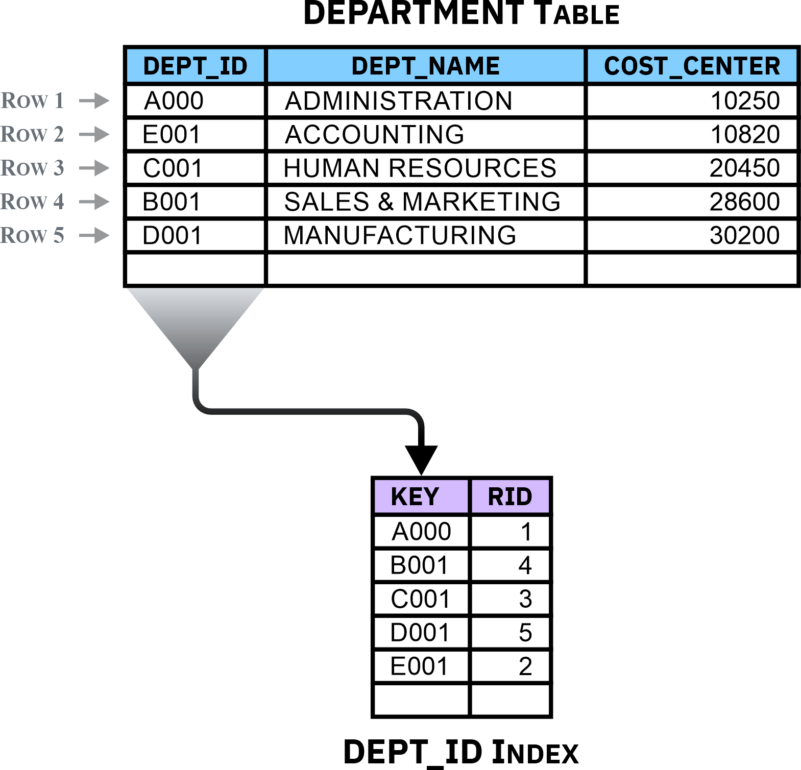
The following illustration shows the structure of a simple index, along with its relationship to the table it derives its data from.

Figure 3: A simple index that has a one-column key

Although some indexes are created automatically to support a table’s definition (for example, to enforce unique and primary key constraints), indexes are typically created explicitly using the CREATE INDEX SQL statement. The basic syntax for this statement is:

CREATE < UNIQUE > INDEX [ IndexName ]
ON [ TableName ] ( [ PriColumnName ] < ASC | DESC > , ... ) >
< INCLUDE ( [ SecColumnName ] , ... ) >

where:

•	IndexName	:	Identifies the name to assign to the index that is to be created.
•	TableName	:	Identifies, by name, the table the index is to be created for (and associated with).
•	PriColumnName	:	Identifies, by name, one or more primary columns that are to be part of the key for the index — if the index is a unique index, the combined values of each primary column specified will be used to enforce data uniqueness in the associated table.
•	SecColumnName	:	Identifies, by name, one or more secondary columns whose values are to be stored with the values of the primary columns, but that are not part of the index key — if the index is a unique index, the values of each secondary column specified will not be used to enforce data uniqueness.

If the INCLUDE clause is specified with the CREATE INDEX statement used, data from the secondary columns specified will be appended to the index’s key values. By storing this information in the index (along with key values), the performance of some queries can be greatly improved. That's because if all the data needed to resolve a query can be obtained by accessing the index only, data does not have to be retrieved from the associated table. (If the data needed to resolve a query does not reside solely in an index, both the index and the associated table must be accessed.)

If the UNIQUE clause is specified with the CREATE INDEX statement used, the resulting index will be a unique index that will be used to ensure the associated table does not contain duplicate occurrences of the same values in the columns that make up the index key. If the table the index is to be created for already contains data, uniqueness is checked and enforced at the time Db2 attempts to create the index, and if records with duplicate index key values are found, the index will not be created. On the other hand, if no duplicates exist, the index will be created and uniqueness will be enforced when INSERT and UPDATE operations are performed against the associated table. (Any time uniqueness of the index key is compromised, the insert or update operation will fail and an error will be generated.)

NOTE: If the INCLUDE clause is specified with the CREATE INDEX statement used, the UNIQUE clause must also be provided.

Thus, to create an index named EMPNO_IDX for a table named EMPLOYEES whose key consists of a column named EMPNO and that includes data from a column named LASTNAME, you would execute a CREATE INDEX statement that looks something like this:

CREATE UNIQUE INDEX empno_idx ON employees(empno) INCLUDE (lastname)

A single table can contain a significant number of indexes; however, every index comes at a price. Because indexes store key column and row pointer data, additional storage space is needed for every index used. Furthermore, write performance is negatively affected — each time an INSERT, UPDATE, or DELETE operation is performed against a table with indexes, every index affected must be updated as well to reflect the changes made. Therefore, indexes should be created only when there is a clear performance advantage to having them available.

Indexes are typically used to improve query performance. So, tables that are used for data mining, business intelligence, business warehousing, and by applications that execute many (and often complex) queries but rarely modify data are prime candidates for indexes. Conversely, tables in online transaction processing (OLTP) environments or environments where data throughput is high should use indexes sparingly or avoid them altogether.

Execute the code:

The code in the next cell builds a CREATE INDEX statement and executes it to create an index named EMP_IDX. It then queries the system catalog to verify that EMP_IDX index exists.

Select the code cell below and carefully read through the comments. This will help you understand the actions the code performs.

When you are ready, click on the

button or press Shift+Enter to execute the code.

In [ ]:

#----------------------------------------------------------------------------------------------#
# Create An Index Named EMP_IDX In The Connected Db2 Database                                  #
#----------------------------------------------------------------------------------------------#

# Define And Initialize The Appropriate Variables
sqlStatement = ""                               # Structured Query Language (SQL) Statement
resultSet = False                               # Pointer To A Result Set
errorMsg = ""                                   # Detailed Error Information
columnHeaders = ("INDNAME", "TABNAME")          # Result Set Column Headers Tuple
columnWidths = (10, 12)                         # Result Set Column Widths Tuple
retCode = True                                  # Return Code

# Define The CREATE INDEX Statement To Be Executed
sqlStatement = "CREATE UNIQUE INDEX emp_idx"    # Create An Index Named EMP_IDX
sqlStatement += " ON employee"                  # For The Table Named EMPLOYEE
sqlStatement += " (empno)"                      # Make The Column Named EMPNO The Index Key
sqlStatement += " INCLUDE (name)"               # And Include Data From The Column Named NAME

# Execute The CREATE INDEX Statement Just Defined By Calling The ibm_db.exec_immediate() API
# (This API Prepares And Executes An SQL Statement In A Single Step)
print("Executing the following SQL statement:\n\n" + sqlStatement)
try:
    resultSet = ibm_db.exec_immediate(connectionID, sqlStatement)
except Exception:
    print("\nERROR: Unable to execute the SQL statement specified.\n")    
    pass

# If The SQL Statement Could Not Be Executed, Display A Detailed Error Message And Exit
# (Call The ibm_db.stmt_errormsg() API To Obtain Detailed Error Information)
if resultSet == False:
    errorMsg = ibm_db.stmt_errormsg()
    print(errorMsg + "\n")
    exit(-1)
    
# Otherwise, Print "Done" And Display A Section Divider Line
else:
    print("\nDone!\n")
    print('*' * 100)
    print()
    
#----------------------------------------------------------------------------------------------#
# Retrieve Information About The EMP_IDX Index From The System Catalog                         #
#----------------------------------------------------------------------------------------------#

# Define The SQL Statement To Be Executed
sqlStatement = "SELECT INDNAME, TABNAME"        # Retreive The Data Stored In These Columns,
sqlStatement += " FROM SYSCAT.INDEXES"          # From The SYSCAT.INDEXES View,
sqlStatement += " WHERE INDNAME = 'EMP_IDX'"    # For An Index Named 'EMP_IDX'

# Execute The SQL Statement Just Defined By Calling The runQuery() Function Defined Earlier
# (Pass It The SQL Statement To Be Executed, Along With The Tuples That Contain Column Header
# And Column Width Information)
retCode = runQuery(0, sqlStatement, columnHeaders, columnWidths)

# If The SQL Statement Was Successfully Executed, Add A Blank Line To The End Of The Report
if retCode == True:
    print()

Step 13: Generate Explain data for the simple query again to see if the new index improves query performance

Overview:

Now that we have created an index named EMP_IDX for the EMPLOYEE table, let's capture Explain data for the query "SELECT empno, name FROM employee" again to see if the index will improve help performance.

Execute the code:

The code in the next cell executes the EXPLAIN statement that was used earlier to generate Explain data for the query "SELECT empno, name FROM employee". It then retreives information from the EXPLAIN_STATEMENT Explain table again to see if the cost of the access plan chosen by the Db2 query optimizer is lower.

Select the code cell below and carefully read through the comments. This will help you understand the actions the code performs.

When you are ready, click on the

button or press Shift+Enter to execute the code.

In [ ]:

#----------------------------------------------------------------------------------------------#
# Get Query Execution Time Information From The EXPLAIN_STATEMENT Explain Table                #
#----------------------------------------------------------------------------------------------#

# Define And Initialize The Appropriate Variables
sqlStatement = ""                               # Structured Query Language (SQL) Statement
resultSet = False                               # Pointer To A Result Set
errorMsg = ""                                   # Detailed Error Information
retCode = True                                  # Return Code

# Define The EXPLAIN Statement To Be Executed
sqlStatement = "EXPLAIN ALL FOR"                # Generate Comprehensive Explain Data
sqlStatement += " SELECT empno, name"           # For The SQL Statement "SELECT empno, name
sqlStatement += " FROM employee"                # FROM employee"

# Execute The EXPLAIN Statement Just Defined By Calling The ibm_db.exec_immediate() API
# (This API Prepares And Executes An SQL Statement In A Single Step)
print("Executing the following SQL statement:\n\n" + sqlStatement)
try:
    resultSet = ibm_db.exec_immediate(connectionID, sqlStatement)
except Exception:
    print("\nERROR: Unable to execute the SQL statement specified.\n")    
    pass

# If The SQL Statement Could Not Be Executed, Display A Detailed Error Message And Exit
# (Call The ibm_db.stmt_errormsg() API To Obtain Detailed Error Information)
if resultSet == False:
    errorMsg = ibm_db.stmt_errormsg()
    print(errorMsg + "\n")
    exit(-1)
    
# Otherwise, Print "Done" And Display A Section Divider Line
else:
    print("\nDone!\n")
    print('*' * 100)

#----------------------------------------------------------------------------------------------#
# Retrieve Information From The EXPLAIN_TIME Explain Table That Was Generated When The EXPLAIN #
# SQL Statement Was Executed                                                                   #
#----------------------------------------------------------------------------------------------#

# Initialize The Column Headers Tuple 
columnHeaders = ("STATEMENT_TEXT", "EXPLAIN_TIME", "TOTAL_COST (Timerons)")

# Initialize The Column Widths Tuple 
columnWidths = (75, 12, 21)
    
# Define The SQL Statement To Be Executed
sqlStatement = "SELECT STATEMENT_TEXT,"               # Retreive The Data Stored In This Column,
sqlStatement += " TIME(EXPLAIN_TIME),"                # And This Column (Without The Date)
sqlStatement += " CAST(TOTAL_COST AS DECIMAL(8, 4))"  # And This Column (Cast As A Decimal Value)
sqlStatement += " FROM SYSTOOLS.EXPLAIN_STATEMENT"    # From The SYSTOOLS.EXPLAIN_STATEMENT Table
sqlStatement += " WHERE TOTAL_COST <> 0"              # Where TOTAL_COST Does NOT Equal 0 (Which
                                                      #  Indicates No Access Plan Has Been 
                                                      #  Choosen Yet)

# Execute The SQL Statement Just Defined By Calling The runQuery() Function Defined Earlier
# (Pass It The SQL Statement To Be Executed, Along With The Tuples That Contain Column Header
# And Column Width Information)
retCode = runQuery(2, sqlStatement, columnHeaders, columnWidths)

# If The SQL Statement Was Successfully Executed, Add A Blank Line To The End Of The Report
# And A Message Stating That The EXPLAIN_TIME Value Indicates The "Before" And "After" Index
# Explain Time Values
if retCode == True:
    print()
    print("NOTE: The record with the earliest EXPLAIN_TIME value is associated with ", end="")
    print("the access plan that was generated\n     \033[1m before\33[0m the ", end="")
    print("EMP_IDX index was created; the record with the most recent EXPLAIN_TIME ", end="")
    print("value is associated\n      with the access plan that was generated", end="")
    print("\033[1m after\033[0m the EMP_IDX index was created.\n")

Step 14: Roll back and commit a transaction

Overview:

A transaction (also known as a unit of work) is a sequence of one or more SQL operations that are grouped together as a single unit, usually within an application process. Such units are considered atomic (from the Greek word meaning “not able to be cut”) because they are indivisible — either all of a transaction’s work is carried out, or none of its work is done.

A given transaction can perform any number of SQL operations, depending upon what is considered a single step within a company’s business logic. With that said, it is important to note that the longer a transaction is — that is, the more SQL operations a transaction performs — the more problematic it can be to manage. This is especially true if multiple transactions must run concurrently.

The initiation and termination of a single transaction defines points of consistency within a Db2 database. Consequently, either the effects of all operations performed within a transaction are applied to the database and made permanent (i.e. committed), or they are backed out (rolled back) and the database is returned to the state it was in immediately before the transaction was started.

Normally, a transaction is initiated the first time an SQL statement is executed after a connection to a database has been established, or when an SQL statement is executed after a running transaction has ended. Once started, transactions can be implicitly committed using a feature known as automatic commit (in which case, each executable SQL statement is treated as a single transaction, and changes made by that statement are automatically applied to the database unless the statement fails to execute successfully). Or, they can be explicitly terminated by executing either the COMMIT or the ROLLBACK SQL statement. The basic syntax for these two statements is:

COMMIT < WORK >

ROLLBACK < WORK >

When the COMMIT statement is used to terminate a transaction, all changes made to the database since the transaction began are made permanent. When the ROLLBACK statement is used instead, all changes made are backed out, and the database is returned to the state it was in just before the transaction was started.

Uncommitted changes made by a transaction are usually inaccessible to other users and applications (there are exceptions) and can be backed out at any time. However, once a transaction’s changes have been committed, they become accessible to all users and applications and the only way to remove the changes made is by performing an UPDATE or DELETE operation.

With Python and Jupyter Notebook, the ibm_db.commit( ) and ibm_db.rollback( ) application programming interfaces (APIs) in the ibm_db library can be used to terminate transactions. These APIs eliminate the need to prepare and execute COMMIT and/or ROLLBACK SQL statements. In addition, the ibm_db.autocommit( ) API can be used to determine if automatic commit behavior is enabled or disabled, as well as turn this behavior ON or OFF.

Execute the code:

The code in the next cell executes the ibm_db.autocommit( ) API to determine whether automatic commit behavior is ON or OFF — if this behavior is ON, the ibm_db.autocommit( ) API is executed again to turn it OFF. Then, the code builds and executes an INSERT statement that adds a record to the EMPLOYEE table created earlier and queries the table to verify the record was added — it can see the record because it owns the transaction that performed the INSERT operation. However, in most cases (there are exceptions), other applications will NOT be able to see the record until the transaction is committed.

After verifying the record was added, the code executes the ibm_db.rollback( ) API to back out the change made by the INSERT operation (transaction). Then, it queries the EMPLOYEE table again to confirm the record no longer exists. Next, it executes the INSERT statement once more and executes the ibm_db.commit( ) API to end the transaction and make the change permanent. Then, it queries the EMPLOYEE table again to verify the record exists. Finally, it executes the ibm_db.autocommit( ) API once more to turn automatic commit behavior ON.

Select the code cell below and carefully read through the comments. This will help you understand the actions the code performs. (There are a lot of different actions taking place in this example, so please review the code carefully.)

When you are ready, click on the

button or press Shift+Enter to execute the code.

In [ ]:

#----------------------------------------------------------------------------------------------#
# Control AUTOCOMMIT Behavior And Manage Transactions                                          #
#----------------------------------------------------------------------------------------------#

# Define And Initialize The Appropriate Variables
insertStatement = ""                            # SQL INSERT Statement
queryStatement = ""                             # SQL SELECT Statement
resultSet = False                               # Pointer To A Result Set
connErrorMsg = ""                               # Database Connection Error Information
stmtErrorMsg = ""                               # SQL Statement Error Information
retCode = 0                                     # Return Code
queryRetCode = 0                                # Autocommit API Query Mode Return Code
setRetCode = False                              # Autocommit API Set Mode Return Code

#----------------------------------------------------------------------------------------------#
# Determine AUTOCOMMIT Behavior - If It's ON, Turn It OFF                                      #
#----------------------------------------------------------------------------------------------#

# Determine Whether AUTOCOMMIT Behavior Is Currently ON Or OFF By Calling The
# ibm_db.autocommit() API (AUTOCOMMIT Behavior Should Be ON Since This Behavior Was Enabled
# When The Database Connection Was First Established)
try:
    queryRetCode = ibm_db.autocommit(connectionID)
except Exception:
    print("\nERROR: Unable to determine AUTOCOMMIT behavior setting.\n")  
    connErrorMsg = ibm_db.conn_error(connectionID)
    print(connErrorMsg + "\n")
    exit(-1)

# If Autocommit Behavior Is ON, Turn It OFF By Calling The ibm_db.autocommit() API
# With The Appropriate Value (ibm_db.SQL_AUTOCOMMIT_OFF)
if queryRetCode == 1:    
    print("\nAUTOCOMMIT behavior is currently ON; turning it OFF ... ", end="")
    try:
        setRetCode = ibm_db.autocommit(connectionID, ibm_db.SQL_AUTOCOMMIT_OFF)
    except Exception:
        pass
    
    # If AUTOCOMMIT Behavior Could Not Be Turned OFF, Display An Error Message And Exit
    # (Call The ibm_db.conn_error() API To Obtain Detailed Error Information)    
    if setRetCode == False:
        print("\nERROR: Unable to turn AUTOCOMMIT behavior OFF.\n")  
        connErrorMsg = ibm_db.conn_error(connectionID)
        print(connErrorMsg + "\n")
        exit(-1)      
        
    # Otherwise, Print "Done" And Display A Section Divider Line
    else:
        print("Done!\n")
        print('*' * 100)

# If AUTOCOMMIT Behavior Is OFF, Display A Message Stating That Along With A
# Section Divider Line
elif queryRetCode == 0:
    print("\nAUTOCOMMIT behavior is currently OFF\n")
    print('*' * 100)
    
#----------------------------------------------------------------------------------------------#
# Insert A Record Into The EMPLOYEE Table Created Earlier                                      #
#----------------------------------------------------------------------------------------------#

# Define The INSERT Statement That Is To Be Used To Add Data To The EMPLOYEE Table
insertStatement = "INSERT INTO employee"    # Insert Into The EMPLOYEE Table
insertStatement += " VALUES(1010,"          # The Value 1010 For The EMPNO Column
insertStatement += " 'AUDREY HEPBURN',"     # The Value 'AUDREY HEPBURN' For The NAME Column
insertStatement += " '10/20/2022',"         # The Value '10/20/2022 For The HIREDATE Column
insertStatement += " 'ANALYST',"            # The Value 'ANALYST' For The TITLE Column
insertStatement += " 'E01',"                # The Value 'E01' For The DEPT Column
insertStatement += " 128450.00)"            # And The Value 128450.00 For The SALARY Column

# Execute The INSERT Statement Just Defined By Calling The ibm_db.exec_immediate() API
# (This API Prepares And Executes An SQL Statement In A Single Step)
print("\nExecuting the following INSERT statement:\n\n" + insertStatement)
try:
    resultSet = ibm_db.exec_immediate(connectionID, insertStatement)
except Exception:
    print("\nERROR: Unable to execute the INSERT statement specified.\n")    
    pass

# If The INSERT Statement Could Not Be Executed, Display A Detailed Error Message And Exit
# (Call The ibm_db.stmt_errormsg() API To Obtain Detailed Error Information)
if resultSet == False:
    errorMsg = ibm_db.stmt_errormsg()
    print(errorMsg + "\n")
    exit(-1)

# Otherwise, Print "Done" And Display A Section Divider Line
else:
    print("\nDone!\n")
    print('*' * 100)
    
#----------------------------------------------------------------------------------------------#
# Query The EMPLOYEE Table To Comfirm That The INSERT Statement Was Executed Successfully      #
# (We Can See The Record Because We're Still In The Transaction That Inserted It; Other Users  #
# CANNOT See The Record Unless They Are Running Under The 'Uncommitted Read' Isolation Level)  #
#----------------------------------------------------------------------------------------------#

# Define The SELECT Statement That Is To Be Executed
selectStatement = "SELECT * FROM employee"        # Retreive All Data From The EMPLOYEE Table
selectStatement += " WHERE empno = 1010"          # For The Record With An EMPNO Value Of 1010

# Define And Initialize A Column Headers Tuple 
columnHeaders = ("EMPNO", "NAME", "HIREDATE", "TITLE", "DEPT", "SALARY")

# Define And Initialize A Column Widths Tuple 
columnWidths = (5, 18, 10, 15, 4, 10)

# Execute The SELECT Statement Just Defined By Calling The runQuery() Function Defined Earlier
# (Pass It The SQL Statement To Be Executed, Along With The Tuples That Contain Column Header
# And Column Width Information)
retCode = runQuery(0, selectStatement, columnHeaders, columnWidths)

# If The SQL Statement Was Successfully Executed, Add A Blank Line To The End Of The Report
if retCode == True:
    print()
    print('*' * 100)
    
#----------------------------------------------------------------------------------------------#
# Perform A ROLLBACK Operation To Back Out The Change Just Made                                #
#----------------------------------------------------------------------------------------------#

# Back Out The Change Just Made To The Database By Calling The ibm_db.rollback() API
print("\nBacking out changes made to the database ... ", end="")
resultSet = False
try:
    resultSet = ibm_db.rollback(connectionID)
except Exception:
    print("\nERROR: Unable to roll back the previous operation.")
    pass

# If The Roll Back Operation Could Not Be Performed, Display An Error Message And Exit
# (Call The ibm_db.conn_error() API To Obtain Detailed Error Information)    
if resultSet == False:
    connErrorMsg = ibm_db.conn_error(connectionID)
    print(connErrorMsg + "\n")
    exit(-1)

# Otherwise, Print "Done" And Display A Section Divider Line
else:
    print("Done!\n")
    print('*' * 100)  
    
#----------------------------------------------------------------------------------------------#
# Query The EMPLOYEE Table Again To Comfirm The Change Made By The INSERT Statement Was NOT    #
# Applied To The Database (Because The Transaction Was Rolled Back)                            #
#----------------------------------------------------------------------------------------------#

# Execute The SELECT Statement Again By Calling The runQuery() Function Defined Earlier
# (Pass It The SQL Statement To Be Executed, Along With The Tuples That Contain Column Header
# And Column Width Information)
retCode = runQuery(0, selectStatement, columnHeaders, columnWidths)

# If The SQL Statement Was Successfully Executed, Add A Blank Line To The End Of The Report
if retCode == True:
    print()
    print('*' * 100)
    
#----------------------------------------------------------------------------------------------#
# Insert The Record Into The EMPLOYEE Table Again                                              #
#----------------------------------------------------------------------------------------------#    
    
# Execute The INSERT Statement Again By Calling The ibm_db.exec_immediate() API
# (This API Prepares And Executes An SQL Statement In A Single Step)
print("\nExecuting the following INSERT statement again:\n\n" + insertStatement)
resultSet = False
try:
    resultSet = ibm_db.exec_immediate(connectionID, insertStatement)
except Exception:
    print("\nERROR: Unable to execute the INSERT statement specified.\n")    
    pass

# If The INSERT Statement Could Not Be Executed, Display A Detailed Error Message And Exit
# (Call The ibm_db.stmt_errormsg() API To Obtain Detailed Error Information)
if resultSet == False:
    errorMsg = ibm_db.stmt_errormsg()
    print(errorMsg + "\n")
    exit(-1)

# Otherwise, Print "Done" And Display A Section Divider Line
else:
    print("\nDone!\n")
    print('*' * 100)

#----------------------------------------------------------------------------------------------#
# Commit The Change Just Made                                                                  #
#----------------------------------------------------------------------------------------------#

# Make The Change Just Made To The Database Permanent By Calling The ibm_db.commit() API
print("\nCommitting changes made to the database ... ", end="")
resultSet = False
try:
    resultSet = ibm_db.commit(connectionID)
except Exception:
    print("\nERROR: Unable to commit the previous operation.")
    pass

# If The Commit Operation Could Not Be Performed, Display An Error Message And Exit
# (Call The ibm_db.conn_error() API To Obtain Detailed Error Information)    
if resultSet == False:
    connErrorMsg = ibm_db.conn_error(connectionID)
    print(connErrorMsg + "\n")
    exit(-1)

# Otherwise, Print "Done" And Display A Section Divider Line
else:
    print("Done!\n")
    print('*' * 100)  
    
#----------------------------------------------------------------------------------------------#
# Query The EMPLOYEE Table Once More To Comfirm The Change Made By The INSERT Statement Was    #
# Successfully Applied To The Database (Because The Transaction Was Committed)                 #
#----------------------------------------------------------------------------------------------#

# Execute The SELECT Statement Once More By Calling The runQuery() Function Defined Earlier
# (Pass It The SQL Statement To Be Executed, Along With The Tuples That Contain Column Header
# And Column Width Information)
retCode = runQuery(0, selectStatement, columnHeaders, columnWidths)

# If The SELECT Statement Was Successfully Executed, Add A Blank Line And Display A Section 
# Divider Line
if retCode == True:
    print()
    print('*' * 100) 
        
#----------------------------------------------------------------------------------------------#
# Turn AUTOCOMMIT Behavior ON                                                                  #
#----------------------------------------------------------------------------------------------#    

# Turn AUTOCOMMIT Behavior ON
print("\nTurning AUTOCOMMIT behavior ON ... ", end="")
try:
    setRetCode = ibm_db.autocommit(connectionID, ibm_db.SQL_AUTOCOMMIT_OFF)
except Exception:
    print("\nERROR: Unable to turn AUTOCOMMIT behavior ON.\n") 
    pass
    
# If AUTOCOMMIT Behavior Could Not Be Turned ON, Display An Error Message And Exit
# (Call The ibm_db.conn_error() API To Obtain Detailed Error Information)    
if setRetCode == False:
    connErrorMsg = ibm_db.conn_error(connectionID)
    print(connErrorMsg + "\n")
    exit(-1)      
        
# Otherwise, Print "Done"
else:
    print("Done!\n")

Section 3. Advanced topics

Step 1: Create two User Defined Functions

Overview:

User defined functions (UDFs) are special objects that can be used to extend and enhance the support provided by the built-in functions available with Db2. But, unlike built-in functions, UDFs can take advantage of operating system calls and the Db2 administrative application programming interfaces (APIs) Db2 provides. Several different types of UDFs can be created:

SQL scalar: A function whose body is written entirely in SQL and Db2 SQL Procedural Language (SQL PL) that returns a single value each time it is called. (SQL PL is a language extension of SQL that consists of statements and language elements that can be used to implement procedural logic in user defined functions and stored procedures. You can learn more about SQL PL here: SQL Procedural Language (SQL PL).)
SQL table: A function whose body is written entirely in SQL and SQL PL that returns a result set, in the form of a table, each time it is called.).
Sourced (or Template): A function that is based on another function (referred to as the source function) that already exists. Sourced functions can be columnar, scalar, or tabular in nature; they can also be designed to overload specific operators such as +, –, *, and /. When a sourced function is invoked, all arguments passed to it are converted to the data types the underlying source function expects, and the source function itself is executed. Upon completion, the source function performs any conversions necessary on the results produced and then returns them to the calling application.
External scalar: A function whose body is written in a high-level programming language like C, C++, or Java that returns a single value each time it is called. The function itself resides in an external library and is registered in the database, along with any related attributes.
External table: A function whose body is written in a high-level programming language that returns a result set, in the form of a table, each time it is called. As with external scalar functions, the function itself resides in an external library and is registered in the database, along with any related attributes.
OLE DB External Table: A function whose body is written in a high-level programming language that can access data from an Object Linking and Embedding Database (OLE DB) provider and return a result set in the form of a table.

Once a UDF is created (and registered with a database), it can be used anywhere a comparable built-in function can be used — UDFs are created (and registered with a database) using the CREATE FUNCTION SQL statement. Several forms of this statement are available; the appropriate form to use is determined by the function type desired. The basic syntax for the form of this statement that is used to create an SQL scalar function is:

CREATE FUNCTION [ FunctionName ]
(< < ParameterType > [ ParameterName ] [ DataType ] , ... > )
RETURNS [ OutputDataType ]
< LANGUAGE SQL >
< READS SQL DATA | CONTAINS SQL | MODIFIES SQL DATA >
[ < BEGIN ATOMIC > SQLStatements ; < END > ]
RETURN [ ReturnStatement ]

Similarly, the basic syntax for the form of the CREATE FUNCTION statement that is used to create an SQL table function is:

CREATE FUNCTION [ FunctionName ]
(< < ParameterType > [ ParameterName ] [ DataType ] , ... > )
RETURNS TABLE ( [ ColumnName ] [ ColumnDataType ] , ... )
< LANGUAGE SQL >
< READS SQL DATA | CONTAINS SQL | MODIFIES SQL DATA >
[ < BEGIN ATOMIC > SQLStatements ; < END > ]
RETURN [ ReturnStatement ]

where:

•	FunctionName	:	Identifies the name to assign to the function that is to be created.
•	ParameterType	:	Indicates whether the parameter specified in the *ParameterName* parameter is an input parameter (IN), an output parameter (OUT), or both an input and an output parameter (INOUT).
•	ParameterName	:	Identifies the name to assign to one or more function parameters.
•	DataType	:	Identifies the data type of the parameter specified in the *ParameterName* parameter. (You can learn more about the data types available with Db2 here: Data types)
•	OutputDataType	:	Identifies the data type the function is expected to return.
•	ColumnName	:	Identifies one or more names to assign to the column(s) the function is expected to return (if the function is an SQL table function).
•	ColumnDataType	:	Identifies the data type the function expects to return for each column specified in the *ColumnName* parameter.
•	SQLStatements	:	Identifies one or more SQL statements that are to be executed when the function is invoked — if two or more statements are used, they should be enclosed with the keywords BEGIN ATOMIC and END and each statement must be terminated with a semicolon (;).
•	ReturnStatement	:	Identifies the RETURN statement that is to be used to return data to the user, application, or SQL statement that invoked the function.

The < CONTAINS SQL | READS SQL DATA | MODIFIES SQL DATA > clause identifies the types of SQL statements that can be used in the body of the function: if the CONTAINS SQL clause is specified, the function cannot contain SQL statements that read or modify data, if the READS SQL DATA clause is specified, the function cannot contain SQL statements that modify data; and if the MODIFIES SQL DATA clause is specified, the function can contain SQL statements that both read and modify data.

Thus, to create an SQL scalar function named CONVERT_CTOF( ) that accepts a temperature value in degrees Celsius as input and returns a corresponding temperature value in degrees Fahrenheit, you would execute a CREATE FUNCTION statement that looks something like this:

CREATE FUNCTION convert_ctof (IN temp_c FLOAT) RETURNS FLOAT RETURN FLOAT((temp_c * 1.8) + 32)

On the other hand, to create an SQL table function named DEPT_EMPLOYEES( ) that accepts a department code as input and returns a result set, in the form of a table, that contains basic information about every employee who works in the department specified, you would execute a CREATE FUNCTION statement that looks more like this:

CREATE FUNCTION dept_employees (deptno CHAR(3)) RETURNS TABLE (empno INTEGER, name VARCHAR(30)) LANGUAGE SQL READS SQL DATA BEGIN ATOMIC RETURN SELECT empno, name FROM employee AS e WHERE e.dept = dept_employees.deptno; END

Execute the code:

The code in the next cell executes both of the CREATE FUNCTION statements provided as examples. It then queries the system catalog to verify that both functions exist.

Select the code cell below and carefully read through the comments. This will help you understand the actions the code performs.

When you are ready, click on the

button or press Shift+Enter to execute the code.

In [ ]:

#----------------------------------------------------------------------------------------------#
# Create An SQL Scalar User Defined Function (UDF) And An SQL Table UDF                        #
#----------------------------------------------------------------------------------------------#

# Define And Initialize The Appropriate Variables
sqlStatement = ""                               # Structured Query Language (SQL) Statement
resultSet = False                               # Pointer To A Result Set
errorMsg = ""                                   # Detailed Error Information
retCode = True                                  # Return Code

#----------------------------------------------------------------------------------------------#
# Create An SQL Scalar User Defined Function Named CONVERT_CTOF()                              #
#----------------------------------------------------------------------------------------------#

# Display A Message Indicating An SQL Scalar Function Is Being Created
print("\nBUILDING AN SQL SCALAR USER DEFINED FUNCTION")
print('-' * 44)
print()

# Define The CREATE FUNCTION Statement To Be Executed
sqlStatement = "CREATE OR REPLACE FUNCTION"     # Create A Function
sqlStatement += " convert_ctof"                 # Named CONVERT_CTOF()
sqlStatement += " (IN temp_c FLOAT)"            # That Receives A Floating Point Number As Input
sqlStatement += " RETURNS FLOAT"                # And Returns A Floating Point Number As Output
sqlStatement += " RETURN"                       # That After Execution, Returns
sqlStatement += " FLOAT((temp_c * 1.8) + 32)"   # The Value Of The Number Received As Input
                                                #   Multiplied By 1.8 And Then Increased By 32
        
# Execute The CREATE FUNCTION Statement Just Defined By Calling The ibm_db.exec_immediate() API
# (This API Prepares And Executes An SQL Statement In A Single Step)
print("Executing the following SQL statement:\n\n" + sqlStatement)
try:
    resultSet = ibm_db.exec_immediate(connectionID, sqlStatement)
except Exception:
    print("\nERROR: Unable to execute the SQL statement specified.\n")    
    pass

# If The CREATE FUNCTION Statement Could Not Be Executed, Display A Detailed Error Message
# And Exit (Call The ibm_db.stmt_errormsg() API To Obtain Detailed Error Information)
if resultSet == False:
    errorMsg = ibm_db.stmt_errormsg()
    print(errorMsg + "\n")
    exit(-1)
    
# Otherwise, Print "Done" And Display A Section Divider Line
else:
    print("\nDone!\n")
    print('*' * 100)
      
#----------------------------------------------------------------------------------------------#
# Create A SQL Table User Defined Function Named DEPT_EMPLOYEES()                              #
#----------------------------------------------------------------------------------------------#
        
# Display A Message Indicating An SQL Table Function Is Being Created
print("\nBUILDING AN SQL TABLE USER DEFINED FUNCTION")
print('-' * 43)
print()

# Define The CREATE FUNCTION Statement To Be Executed
sqlStatement = "CREATE OR REPLACE FUNCTION"   # Create A Function
sqlStatement += " dept_employees"             # Named DEPT_EMPLOYEES()
sqlStatement += " (deptno CHAR(3))"           # That Receives A 3-Character Code As Input
sqlStatement += " RETURNS TABLE"              # And Returns A Table
sqlStatement += " (empno INTEGER,"            # With A Column Named EMPNO That Holds Integers
sqlStatement += " name VARCHAR(30))"          # And A Column Named NAME That Holds 30 Characters
sqlStatement += " LANGUAGE SQL"               # Whose Body Is Written In SQL and SQL PL
sqlStatement += " READS SQL DATA"             # And Reads, But Does Not Modify Data
sqlStatement += " BEGIN ATOMIC"               #  (This Marks The Start Of Several Statements)
sqlStatement += " RETURN"                     # And That After Execution, Returns The Results
                                              #  Of The Following Query:
sqlStatement += " SELECT empno, name"         # Retreive The Data Stored In These Columns
sqlStatement += " FROM employee AS e"         # From The EMPLOYEE Table (Referenced As E)
sqlStatement += " WHERE e.dept = "            # Where Values In The DEPT Column Of The EMPLOYEE
sqlStatement += " dept_employees.deptno;"     #  Table Match The Values Of The DEPTNO Value
                                              #  Provided To This Function As Input
sqlStatement += " END"                        #  (This Marks The End Of Several Statements)
               
# Execute The CREATE FUNCTION Statement Just Defined By Calling The ibm_db.exec_immediate() API
# (This API Prepares And Executes An SQL Statement In A Single Step)
resultSet = False
print("Executing the following SQL statement:\n\n" + sqlStatement)
try:
    resultSet = ibm_db.exec_immediate(connectionID, sqlStatement)
except Exception:
    print("\nERROR: Unable to execute the SQL statement specified.\n")    
    pass

# If The SQL Statement Could Not Be Executed, Display A Detailed Error Message And Exit
# (Call The ibm_db.stmt_errormsg() API To Obtain Detailed Error Information)
if resultSet == False:
    errorMsg = ibm_db.stmt_errormsg()
    print(errorMsg + "\n")
    exit(-1)
    
# Otherwise, Print "Done" And Display A Section Divider Line
else:
    print("\nDone!\n")
    print('*' * 100)
    
#----------------------------------------------------------------------------------------------#
# Retrieve Information About The Two Functions Just Created From The System Catalog            #
#----------------------------------------------------------------------------------------------#

# Initialize The Result Set Column Headers And Column Widths Tuples
columnHeaders = ("ROUTINE_NAME", "CREATE_TIME")
columnWidths = (14, 26)

# Define The SQL Statement To Be Executed
sqlStatement = "SELECT ROUTINENAME,"            # Retreive The Data Stored In This Column
sqlStatement += " CREATE_TIME"                  # And The Data Stored In This Column
sqlStatement += " FROM SYSCAT.ROUTINES"         # From The SYSCAT.ROUTINES View
sqlStatement += " WHERE ROUTINETYPE = 'F'"      # Where The ROUTINETYPE Column Value Indicates
                                                #  FUNCTION
sqlStatement += " AND ROUTINENAME"              # And The Routine Name
sqlStatement += " = 'CONVERT_CTOF'"             # Is 'CONVERT_CTOF'
sqlStatement += " OR ROUTINENAME"               # Or The Routine Name
sqlStatement += " LIKE 'DEPT_%'"                # Starts With 'DEPT_'
sqlStatement += " ORDER BY CREATE_TIME ASC"     # Arrange Records By Creation Time In 
                                                #  Ascending Order    

# Execute The SQL Statement Just Defined By Calling The runQuery() Function Defined Earlier
# (Pass It The SQL Statement To Be Executed, Along With The Tuples That Contain Column Header
# And Column Width Information)
retCode = runQuery(0, sqlStatement, columnHeaders, columnWidths)

# If The SQL Statement Was Successfully Executed, Add A Blank Line To The End Of The Report
if retCode == True:
    print()

Step 2: Invoke the User Defined Functions created earlier

Overview:

The way in which a user defined function (UDF) can be used is largely dependent upon the function type. A scalar function optionally accepts arguments and returns a single scalar value each time the function is called. Therefore, and SQL scalar function can be used wherever an expression can be used. (An expression is a specification, which can include operators, operands, and parentheses, that a Db2 database can evaluate to one or more values, or to a reference to some database object.)

Table functions, on the other hand, return rows and columns of data much like a table created with a simple CREATE TABLE statement would return when queried. Consequently, a table function can be used only in the FROM clause of an SQL statement.

Execute the code:

The code in the next cell creates and populates a table named WEATHER. Then, it then builds and executes SQL statements that illustrate how each of the user defined functions (UDFs) created in the previous step might be used.

Select the code cell below and carefully read through the comments. This will help you understand the actions the code performs.

When you are ready, click on the

button or press Shift+Enter to execute the code.

In [ ]:

#----------------------------------------------------------------------------------------------#
# Invoke The User Defined Functions Created In The Previous Step                               #
#----------------------------------------------------------------------------------------------#

# Define And Initialize The Appropriate Variables
sqlStatement = ""                               # Structured Query Language (SQL) Statement
resultSet = False                               # Pointer To A Result Set
errorMsg = ""                                   # Detailed Error Information
loopCounter = 1                                 # WHILE Loop Counter Variable
retCode = True                                  # Return Code

#----------------------------------------------------------------------------------------------#
# Create And Populate A Table Named WEATHER                                                    #
#----------------------------------------------------------------------------------------------#

# Define The CREATE TABLE Statement To Be Executed
sqlStatement = "CREATE TABLE weather (" # Create A Table Named WEATHER
sqlStatement += "region CHAR(15), "     # With A Column Named REGION That Accepts 15 Characters
sqlStatement += "avg_temp_c FLOAT) "    # And A Column Named AVG_TEMP_C That Accepts Floating
                                        #  Point Numbers

# Execute The CREATE TABLE Statement Just Defined By Calling The ibm_db.exec_immediate() API
# (This API Prepares And Executes An SQL Statement In A Single Step)
resultSet = False
try:
    resultSet = ibm_db.exec_immediate(connectionID, sqlStatement)
except Exception:
    print("\nERROR: Unable to execute the SQL statement: " + sqlStatement + "\n")    
    pass

# If The CREATE TABLE Statement Could Not Be Executed, Display A Detailed Error Message And
# Exit (Call The ibm_db.stmt_errormsg() API To Obtain Detailed Error Information)
if resultSet == False:
    errorMsg = ibm_db.stmt_errormsg()
    print(errorMsg + "\n")
    exit(-1)

# Populate The Table Just Created By Executing An INSERT Statement 3 Times
while loopCounter <= 3:
    
    # Define The INSERT Statement To Be Used To Add Data To The WEATHER Table
    sqlStatement = "INSERT INTO weather"       # Insert Into The WEATHER Table
    
    # If This Is The First Pass Through The Loop, ...
    if loopCounter == 1:
        sqlStatement += " VALUES('MOUNTAINS'," # The Value 'MOUNTAINS' For The REGION Column
        sqlStatement += " 16)"                 # And The Value 16 The AVG_TEMP_C Column
        
    # If This Is The Second Pass Through The Loop, ...
    if loopCounter == 2:
        sqlStatement += " VALUES('PIEDMONT',"  # The Value 'PIEDMONT' For The REGION Column
        sqlStatement += " 22)"                 # And The Value 22 The AVG_TEMP_C Column
        
    # If This Is The Third Pass Through The Loop, ...
    if loopCounter == 3:
        sqlStatement += " VALUES('COAST',"     # The Value 'COAST' For The REGION Column
        sqlStatement += " 24)"                 # And The Value 24 The AVG_TEMP_C Column
        
    # Execute The INSERT Statement Just Defined By Calling The ibm_db.exec_immediate() API
    # (This API Prepares And Executes An SQL Statement In A Single Step)
    resultSet = False
    try:
        resultSet = ibm_db.exec_immediate(connectionID, sqlStatement)
    except Exception:
        print("\nERROR: Unable to execute the SQL statement: " + sqlStatement + "\n")     
        pass

    # If The INSERT Statement Could Not Be Executed, Display A Detailed Error Message
    # And Exit (Call The ibm_db.stmt_errormsg() API To Obtain Detailed Error Information)
    if resultSet == False:
        errorMsg = ibm_db.stmt_errormsg()
        print(errorMsg + "\n")
        exit(-1)
        
    #Increment The Loop Counter Variable
    loopCounter += 1
    
#----------------------------------------------------------------------------------------------#
# Query The WEATHER Table Using The CONVERT_CTOF() SQL Scalar UDF Created Earlier              #
#----------------------------------------------------------------------------------------------#

# Display A Message Indicating The SQL Scalar Function Created Earlier Is Being Used
print("\nUSING THE SQL SCALAR USER DEFINED FUNCTION NAMED CONVERT_CTOF()")
print('-' * 63)

# Define The SELECT Statement That Is To Be Executed
sqlStatement = "SELECT region,"              # Retreive REGION Data
sqlStatement += " avg_temp_c,"               # And AVG_TEMP_C Data
sqlStatement += " convert_ctof(avg_temp_c)"  # And AVG_TEMP_C Data Converted To Fahrenheit
sqlStatement += " FROM weather"              # From The WEATHER Table

# Initialize The Result Set Column Headers And Column Widths Tuples
columnHeaders = ("REGION", "AVG_TEMP_C", "AVG_TEMP_F")
columnWidths = (12, 12, 12)

# Execute The SELECT Statement Just Defined By Calling The runQuery() Function Defined Earlier
# (Pass It The SQL Statement To Be Executed, Along With The Tuples That Contain Column Header
# And Column Width Information)
retCode = runQuery(0, sqlStatement, columnHeaders, columnWidths)
  
# If The SQL Statement Was Successfully Executed, Print A Blank Line And Display Another
# Section Divider Line
if retCode == True:
    print()
    print('*' * 100)
    
#----------------------------------------------------------------------------------------------#
# Display The Data Returned By The DEPT_EMPLOYEES() SQL Table UDF Created Earlier              #
#----------------------------------------------------------------------------------------------#

# Display A Message Indicating The SQL Table Function Created Earlier Is Being Used
print("\nUSING THE SQL TABLE USER DEFINED FUNCTION NAMED DEPT_EMPLOYEES()")
print('-' * 64)    

# Define The SELECT Statement That Is To Be Executed
sqlStatement = "SELECT empno, name"                  # Retreive The Data Stored In These Columns  
sqlStatement += " FROM TABLE(dept_employees('C01'))" # From The Table Produced When The SQL
                                                     #  Table Function DEPT_EMPLOYEES() Is
                                                     #  Called With The Input Value 'C01'                                                   
sqlStatement += " AS results"                        # And Lable The Data Returned 'results'

# Initialize The Result Set Column Headers And Column Widths Tuples
columnHeaders = ("EMPNO", "NAME")
columnWidths = (6, 18)

# Execute The SELECT Statement Just Defined By Calling The runQuery() Function Defined Earlier
# (Pass It The SQL Statement To Be Executed, Along With The Tuples That Contain Column Header
# And Column Width Information)
retCode = runQuery(0, sqlStatement, columnHeaders, columnWidths)

# If The SQL Statement Was Successfully Executed, Add A Blank Line To The End Of The Report
if retCode == True:
    print()

Step 3: Create an SQL procedure

Overview

Every time an SQL statement is executed against a Db2 database that resides on a remote server, the statement itself is sent over a network to the server for processing. The database at the server then executes the statement and returns the results, again over the network, to the appropriate user/application. This means that two messages must travel over the network for every SQL statement that gets executed. By breaking monolithic applications into separate parts and storing those parts that perform a relatively large amount of database activity with little or no user interaction directly on the database server itself (in the form of a stored procedure), the amount of data that needs to flow across the network can be greatly reduced. In some cases, this approach can also enhance application performance, since the portions of the code that interact with the database are physically stored on the server where computing power and centralized control can deliver quick, coordinated data access.

Stored procedures allow work that is done against a database to be encapsulated and stored in such a way that it can be executed directly at the database server by any application or user who has the appropriate authority. And, because only one SQL statement is needed to invoke a stored procedure (the CALL statement), fewer messages are transmitted across the network — only the data that is actually needed at the client is sent across. It is also important to note that when a stored procedure is used to implement a specific business rule, the logic needed to apply that rule can be incorporated into any application simply by invoking the procedure. Thus, the same business rule logic is guaranteed to be enforced across multiple applications. And if business rules change, only the logic in the procedure has to be modified — applications that call the procedure do not have to be altered.

Two different types of stored procedures can be created:

SQL (or Native SQL): A stored procedure whose body is written entirely in SQL or SQL Procedural Language (SQL PL). (SQL PL is a language extension of SQL that consists of statements and language elements that can be used to implement procedural logic in user defined functions and stored procedures. You can learn more about SQL PL here: SQL Procedural Language (SQL PL).)
External: A stored procedure whose body is written in a high-level programming language such as Assembler, C, C++, COBOL, Java, REXX, or PL/I that resides in an external library that is accessible to DB2; external stored procedures must be registered in a database, along with all their related attributes, before they can be invoked.

While SQL procedures offer rapid application development and considerable flexibility, external stored procedures can be much more powerful because they can exploit system calls and the administrative application programming interfaces (APIs) that are provided with Db2. However, this increase in functionality makes them much more difficult to produce. In fact, the following steps are required to create an external stored procedure:

Construct the body of the procedure, using a supported high-level programming language.
Compile and link the procedure to create a shared (dynamic-link) library.
Debug the procedure, repeating steps 1 and 2 until all problems have been resolved.
Physically store the library containing the procedure on the database server.
Modify system permissions for the library so that all users with the proper authority can execute it.
Register the procedure with the appropriate Db2 database (running on the server).

Regardless of whether stored procedures are written using SQL or a high-level programming language, they must perform the following tasks, in the order shown:

Accept any input parameter values the calling application supplies.
Perform whatever processing is appropriate (typically, this involves executing one or more SQL statements as a single operation).
Return output data (if data is to be returned) to the calling application — at a minimum, a stored procedure should return a value that indicates whether it executed successfully.

Stored procedures are created by executing the CREATE PROCEDURE statement. Two forms of this statement are available, and the appropriate form to use is determined by the stored procedure type. The basic syntax for the form of the CREATE PROCEDURE statement that is used to create an SQL stored procedure looks something like this:

CREATE PROCEDURE [ ProcedureName ]
(< < ParameterType > [ ParameterName ] [ DataType ] , ... > )
< LANGUAGE SQL >
< DYNAMIC RESULT SETS [ 0 | NumResultSets ] >
< READS SQL DATA | CONTAINS SQL | MODIFIES SQL DATA >
[ < BEGIN ATOMIC > SQLStatements ; < END > ]

where:

•	ProcedureName	:	Identifies the name to assign to the procedure that is to be created.
•	ParameterType	:	Indicates whether the parameter specified in the *ParameterName* parameter is an input parameter (IN), an output parameter (OUT), or both an input and an output parameter (INOUT).
•	ParameterName	:	Identifies the name to assign to one or more function parameters.
•	DataType	:	Identifies the data type of the parameter specified in the *ParameterName* parameter. (You can learn more about the data types available with Db2 here: Data types)
•	NumResultSets	:	Identifies the number of result sets the procedure returns (if any).
•	SQLStatements	:	Identifies one or more SQL statements that are to be executed when the procedure is invoked — if two or more statements are used, they should be enclosed with the keywords BEGIN and END and each statement must be terminated with a semicolon (;).

Thus, to create an SQL procedure named HIGH_EARNERS( ) that returns a list of employees whose salary exceeds the average salary (in the form of a result set), along with the average employee salary, you might execute a CREATE PROCEDURE statement that looks something like this:

CREATE PROCEDURE high_earners (OUT avg_salary FLOAT) LANGUAGE SQL DYNAMIC RESULT SETS 1 READS SQL DATA BEGIN DECLARE c1 CURSOR WITH RETURN FOR SELECT name, salary FROM employee WHERE salary > avg_salary ORDER BY salary DESC; DECLARE EXIT HANDLER FOR NOT FOUND SET avg_salary = 0; SET avg_salary = 0; SELECT AVG(salary) INTO avg_salary FROM employee; OPEN c1; END

When this particular CREATE PROCEDURE statement is executed, the SQL procedure produced will return an integer value (in an output parameter called AVG_SALARY) and a result set that contains the name and salary of each employee whose salary is higher than the average salary paid to employees. Key elements that control this behavior include:

Specifying the DYNAMIC RESULT SETS 1 clause with the CREATE PROCEDURE statement used, indicating the SQL procedure is to return a one result set.
Defining a cursor within the procedure body (and specifying the WITH RETURN FOR clause in the DECLARE CURSOR statement used) so a result data set will be returned.
Querying the EMPLOYEE table using the built-in AVG( ) scalar function to obtain average salary information.
Opening the cursor (which causes the query that obtains employee salary information to be executed and a result data set to be produced).
Returning the average salary to the calling statement (in the output parameter named AVGSALARY) and leaving the cursor that was created open so the data in the result set produced can be accessed by the calling application.

Execute the code:

The code in the next cell executes the CREATE PROCEDURE statement that was provided as an example. It then queries the system catalog to verify that the procedure exists.

Select the code cell below and carefully read through the comments. This will help you understand the actions the code performs.

When you are ready, click on the

button or press Shift+Enter to execute the code.

In [ ]:

#----------------------------------------------------------------------------------------------#
# Create An SQL Procedure                                                                      #
#----------------------------------------------------------------------------------------------#

# Define And Initialize The Appropriate Variables
sqlStatement = ""                               # Structured Query Language (SQL) Statement
resultSet = False                               # Pointer To A Result Set
errorMsg = ""                                   # Detailed Error Information
retCode = True                                  # Return Code

# Display A Message Indicating An SQL Procedure Is Being Created
print("\nBUILDING AN SQL PROCEDURE")
print('-' * 25)
print()

# Define The CREATE PROCEDURE Statement To Be Executed       
sqlStatement = "CREATE OR REPLACE"              # Create Or Replace
sqlStatement += " PROCEDURE high_earners"       # A Procedure Named HIGH_EARNERS()
sqlStatement += " (OUT avg_salary FLOAT)"       # That Returns An Integer As Output
sqlStatement += " LANGUAGE SQL"                 # That Is Written In SQL/PL SQL
sqlStatement += " DYNAMIC RESULT SETS 1"        # And That Returns 1 Result Set
sqlStatement += " READS SQL DATA"               # And Can Read, But Not Update Data
sqlStatement += " BEGIN"                        #  (This Marks The Start Of Several Statements)
sqlStatement += " DECLARE c1 CURSOR"            # Define A Cursor Named C1
sqlStatement += " WITH RETURN FOR"              # That Will Return Data Generated By A Query:
sqlStatement += " SELECT name, salary"          # That Retrieves NAME and SALARY Data
sqlStatement += " FROM employee"                # From The EMPLOYEE Table
sqlStatement += " WHERE salary > avg_salary"    # Where SALARY Is Greater Than The Average
sqlStatement += " ORDER BY salary DESC;"        # And Sorts The Data, By SALARY, Descending

sqlStatement += " DECLARE EXIT HANDLER"         # Define An Exit Handler Such That:
sqlStatement += " FOR NOT FOUND"                # If No Data Is Found,
sqlStatement += " SET avg_salary = 0;"          # An Average SALARY Value Of 0.99 Is Returned

sqlStatement += " SET avg_salary = 0;"          # Set The AVG_SALARY Variable Value To 0

sqlStatement += " SELECT AVG(salary)"           # Use The Function AVG() To Get The Average
sqlStatement += " INTO avg_salary"              # SALARY And Store It In The Output Variable
sqlStatement += " FROM employee;"               # Using Data Found In The EMPLOYEE Table

sqlStatement += " OPEN c1;"                     # Open The C1 Cursor Defined Earlier
sqlStatement += " END"                          #  (This Marks The End Of Several Statements)
        
# Execute The CREATE Procedure Statement Just Defined By Calling The ibm_db.exec_immediate() API
# (This API Prepares And Executes An SQL Statement In A Single Step)
print("Executing the following SQL statement:\n\n" + sqlStatement)
try:
    resultSet = ibm_db.exec_immediate(connectionID, sqlStatement)
except Exception:
    print("\nERROR: Unable to execute the SQL statement specified.\n")    
    pass

# If The CREATE PROCEDURE Statement Could Not Be Executed, Display A Detailed Error Message
# And Exit (Call The ibm_db.stmt_errormsg() API To Obtain Detailed Error Information)
if resultSet == False:
    errorMsg = ibm_db.stmt_errormsg()
    print(errorMsg + "\n")
    exit(-1)
    
# Otherwise, Print "Done" And Display A Section Divider Line
else:
    print("\nDone!\n")
    print('*' * 100)

#----------------------------------------------------------------------------------------------#
# Retrieve Information About The Procedure Just Created From The System Catalog                #
#----------------------------------------------------------------------------------------------#

# Initialize The Result Set Column Headers And Column Widths Tuples
columnHeaders = ("ROUTINE_NAME", "CREATE_TIME")
columnWidths = (14, 26)

# Define The SQL Statement To Be Executed
sqlStatement = "SELECT ROUTINENAME,"            # Retreive The Data Stored In This Column
sqlStatement += " CREATE_TIME"                  # And The Data Stored In This Column
sqlStatement += " FROM SYSCAT.ROUTINES"         # From The SYSCAT.ROUTINES View
sqlStatement += " WHERE ROUTINETYPE = 'P'"      # Where The ROUTINETYPE Column Value Indicates
                                                #  PROCEDURE
sqlStatement += " AND ROUTINENAME"              # And The ROUTINENAME Name
sqlStatement += " = 'HIGH_EARNERS'"             # Is 'HIGH_EARNERS'

# Execute The SQL Statement Just Defined By Calling The runQuery() Function Defined Earlier
# (Pass It The SQL Statement To Be Executed, Along With The Tuples That Contain Column Header
# And Column Width Information)
retCode = runQuery(0, sqlStatement, columnHeaders, columnWidths)

# If The SQL Statement Was Successfully Executed, Add A Blank Line To The End Of The Report
if retCode == True:
    print()

Step 4: Invoke a procedure

Overview

Once a procedure has been created and registered with a database (via the CREATE PROCEDURE statement), it can be invoked by executing the CALL statement. The basic syntax for this statement is:

CALL [ ProcedureName ]
( [ InputParameter ] | [ OutputParameter ] | DEFAULT | NULL , ... )

where:

•	ProcedureName	:	Identifies, by name, the procedure that is to be invoked.
•	InputParameter	:	Identifies one or more values (or application variables containing values) that are to be passed to the procedure as input parameters.
•	OutputParameter	:	Identifies one or more values (or application variables containing values) that are to receive values that will be returned as output from the procedure.

Like other dynamic SQL statements that can be prepared and executed at runtime, CALL statements can contain parameter markers in place of constants and expressions. (You may recall that parameter markers are represented by the question mark character (?) and indicate the position in an SQL statement where the current value of one or more application variables are to be substituted at the time the statement is executed.)

Thus, the SQL procedure named HIGH_EARNERS( ) that was created earlier can be invoked by executing a CALL statement that looks something like this:

CALL high_earners (?)

While the CALL SQL statement can be prepared and executed (using parameter markers) with Python and Jupyter Notebook, there is no way to retrieve any data and/or result set(s) the procedure being called might produce. Instead, the ibm_db.callproc( ) application programming interface (API) in the ibm_db library must be used to invoke procedures when Python or Jupyter Notebook is used. The syntax for this API is:

ibm_db.callproc ( IBM_DBConnection connectionID, string procName [, tuple procParams ] )

where:

• connectionID : Identifies a valid Db2 database connection object (that was created by calling the ibm_db.connect( ) or ibm_db.pconnect( ) API). • procName : Identifies, by name, the procedure that is to be invoked. • procParams : A Python tuple containing values (or value placeholders) for each parameter required by the procedure specified in the procName parameter.

If the execution of this API is successful, an IBM_DBStatement object, (or a tuple containing an IBM_DBStatement object), followed by a potentially modified tuple containing a copy of the parameter values that were supplied for the procPrams parameter when the API was called, will be returned. (Values for IN parameters are left untouched whereas values for OUT and INOUT parameters may have been changed by the procedure.) If the execution of this API is unsuccessful, the value None will be returned instead.

Execute the code:

The code in the next cell executes both the CALL SQL statement and the ibm_db.callproc( ) API to invoke the procedure named HIGH_EARNERS( ) that was created earlier.

Select the code cell below and carefully read through the comments. This will help you understand the actions the code performs.

When you are ready, click on the

button or press Shift+Enter to execute the code.

In [ ]:

#----------------------------------------------------------------------------------------------#
# Invoke The SQL Procedure Created In The Previous Step                                        #
#----------------------------------------------------------------------------------------------#

# Define And Initialize The Appropriate Variables
sqlStatement = ""                               # Structured Query Language (SQL) Statement
preparedStmt = None                             # Pointer To A Prepared SQL Statement
errorMsg = ""                                   # Detailed Error Information
retCode = True                                  # Return Code
procParamValue = (0.0,)                         # SQL Procedure Parameter Value
procName = "HIGH_EARNERS"                       # SQL Procedure Name
resultSet = False                               # Pointer To A Result Set
avgSalary = 0                                   # Average Salary (Returned By Procedure)
noData = False                                  # No Data Found Flag
dataRecord = False                              # Data Record
firstPass = True                                # First Pass Through Record Display Loop Flag
columnHeaders = ("NAME", "SALARY")              # Column Headers Tuple 
columnWidths = (18, 11)                         # Column Widths Tuple 
numRows = 0                                     # Number Of Records (Rows) Retreived 

#----------------------------------------------------------------------------------------------#
# Use The CALL Statement To Invoke The HIGH_EARNERS() Procedure Created Earlier                #
#----------------------------------------------------------------------------------------------#

# Display A Message Indicating The CALL Statement Is Being Used To Invoke The Procedure
# Created Earlier
print("\nUSING THE CALL STATEMENT TO INVOKE THE PROCEDURE NAMED HIGH_EARNERS()")
print('-' * 69)       

#----------------------------------------------------------------------------------------------#
# Prepare The CALL Statement Needed To Invoke The HIGH_EARNERS() Procedure Created Earlier     #
#----------------------------------------------------------------------------------------------#

# Define The CALL Statement That Is To Be Executed
sqlStatement = "CALL high_earners"         # Invoke The Procedure Named HIGH_EARNERS  
sqlStatement += " (?)"                     # With The Parameter Marker For The CODE Column Value
                                                       
# Prepare The CALL Statement Just Defined By Calling The ibm_db.prepare() API
print("\nPreparing the following SQL statement for execution:\n\n" + sqlStatement)
try:
    preparedStmt = ibm_db.prepare(connectionID, sqlStatement)
except Exception:
    print("\nERROR: Unable to prepare the SQL statement specified.\n")
    pass

# If The SQL Statement Could Not Be Prepared, Display A Detailed Error Message And Exit
# (Call The ibm_db.stmt_errormsg() API To Obtain Detailed Error Information)
if preparedStmt == None:
    errorMsg = ibm_db.stmt_errormsg()
    print(errorMsg + "\n")
    exit(-1)
    
# Otherwise, Add A Blank Line To The End Of The Report
else:
    print()
    
#----------------------------------------------------------------------------------------------#
# Execute The CALL Statement Needed To Invoke The HIGH_EARNERS() Procedure Created Earlier     #
#----------------------------------------------------------------------------------------------#
    
# Execute The CALL Statement Prepared Earlier By Calling The ibm_db.execute() API
# (Provide The Current Data Record Tuple As An Input Value)
print("Executing the prepared statement ... ", end="")
try:
    retCode = ibm_db.execute(preparedStmt, procParamValue)
except Exception:
    print("\nERROR: Unable to execute the prepared CALL statement.\n")    
    pass
    
# If The Prepared CALL Statement Could Not Be Executed, Display A Detailed Error Message And Exit
# (Call The ibm_db.stmt_errormsg() API To Obtain Detailed Error Information)
if retCode == False:
    errorMsg = ibm_db.stmt_errormsg()
    print(errorMsg + "\n")
    exit(-1)   
    
# Otherwise, Print "Done" And Display A Section Divider Line
else:
    print("Done!\n")

# Print The Average Salary Information Retrieved
print("Average salary information returned by the HIGH_EARNERS() Procedure: ", end="")
print("${:>10.2f}\n" .format(procParamValue[0]))

# Display A Message Stating The ibm_db.callproc() API Is Required To See The Records
print("NOTE: Even though the\033[1m CALL\33[0m statement executed successfully, ", end="")
print("there is no way to obtain the data\n      produced by this procedure. That's ", end="")
print("why the\033[1m ibm_db.callproc()\33[0m API must be used instead.\n")

# Display A Section Divider
print('*' * 100)

#----------------------------------------------------------------------------------------------#
# Use The ibm_db.callproc() API To Invoke The HIGH_EARNERS() Procedure Created Earlier         #
#----------------------------------------------------------------------------------------------#

# Display A Message Indicating The ibm_db.callproc() API Is Being Used To Invoke The Procedure
# Created Earlier
print("\nUSING THE ibm_db.callproc() API TO INVOKE THE PROCEDURE NAMED HIGH_EARNERS()")
print('-' * 76)

# Invoke The HIGH_EARNERS() Procedure By Calling The ibm_db.callproc() API
try:
    resultSet, avgSalary = ibm_db.callproc(connectionID, procName, procParamValue)
except Exception:
    print("\nERROR: Unable to execute the " + procName + "() procedure.\n")    
    pass

# If The Procedure Could Not Be Executed, Display A Detailed Error Message And Exit
# (Call The ibm_db.sconn_error() API To Obtain Detailed Error Information)
if resultSet == None:
    errorMsg = ibm_db.conn_error(connectionID)
    print(errorMsg + "\n")
    exit(-1)

# Display A Header Label
print("\nEmployees with a salary above the average salary (", end="")

# Display The Average Salary Value Returned By The Procedure    
print("${:>10.2f}) :\n" .format(avgSalary))     

# As Long As There Are Records In The Result Set Produced, ...
while noData == False:

    # Retrieve A Record And Store Its Values In A Tuple By Calling The ibm_db.fetch_tuple() API
    try:
        dataRecord = ibm_db.fetch_tuple(resultSet)
    except:
        print("ibm_db.fetch_tuple() returned an error.\n")
        pass

    # If A Record Could Not Be Retrieved Or If No Record Was Found, Set The "No Data" Flag To TRUE 
    # To Exit The while() Loop
    if dataRecord == False:
        noData = True
       
        # If This Is The First Pass Through The while() Loop,  Display A "No Records Found" 
        # Message And Exit The Loop
        if firstPass == True:
            print("No records found.")
            break

    # Otherwise, Display The Appropriate Information
    else:
            
        # If This Is The First Pass Through The while() Loop, ...
        if firstPass == True:
                
            # Display The Column Headers Provided In The columnHeaders Tuple - Left Justify
            # The Text And Make Each Column The Width Specified In The columnWidths Tuple
            for tupIndx in range(2):
                print(f'{columnHeaders[tupIndx]:<{columnWidths[tupIndx]}}', end="")
                print("  ", end="")      # Space Between Column Header Values           
         
            # Terminate The Line And Display Column Header/Value Dividing Lines Just Below
            # The Column Headers
            print()
            for tupIndx in range(2):
                print(f'{"":-<{columnWidths[tupIndx]}}', end="")
                print("  ", end="")      # Space Between Column Header Dividing Lines  
                    
            # Terminate The Line And Set The "First Pass" Flag To FALSE So Header
            # Information Will Not Be Displayed Again
            print()
            firstPass = False
            
        # Format And Display The Data For Each Record Retreived
        for tupIndx in range(2):         # For Every Column In The Record, ...

            # Copy The Data Value Into A Character String Variable And Remove Any Trailing 
            # Space Characters Found
            dataValue = "{}".format(dataRecord[tupIndx])
            newValue = dataValue.rstrip()

            # If The Data Value Contains A Decimal Point, Add a "$" Symbol To The Front And
            # Display The Value Right Justified, Using The Width Specified In The 
            # columnWidths Tuple (This Is SALARY Data)
            if ("." in dataValue) == True:
                newValue = "$ " + dataValue
                dataValue = newValue.rstrip()
                print(f'{dataValue:>{columnWidths[tupIndx]}}', end="")
               
            # Otherwise (This Is NAME Data), ...
            else:
        
                # Display The Data Value Left Justified, Using The Width Specified
                # In The columnWidths Tuple
                print(f'{newValue:<{columnWidths[tupIndx]}}', end="")
                       
            # Add Spaces Between This Column Value And The Next 
            print("  ", end="")           # Space Between Column Values 
          
        # Terminate The Line And Increment The Records (Rows) Counter
        print()
        numRows = numRows + 1

# If Records Were Retreived, Display The Number Of Records Found And Add A Blank
# Line To The End Of The Report
if firstPass == False:
    print("\nNumber of records (rows) found:", numRows)
    print()

Section 4. Lab environment clean up

Step 1: Remove the tables used by the Db2 EXPLAIN facility (if using IBM Db2 Community Edition)

Overview:

In Step 11 of Section 2, the tables that are needed for the Explain facility were created by calling the SYSPROC.SYSINSTALLOBJECTS( ) stored procedure. As pointed out in Section 10, the SYSPROC.SYSINSTALLOBJECTS( ) procedure is used to both create and drop the database objects that are required by a specific Db2 tool. You may recall that the SQL syntax used to execute this procedure is:

CALL SYSPROC.SYSINSTALLOBJECTS ( [ ToolName ], [ Action ], [ TablespaceName ], [ SchemaName ] )

where:

•	ToolName	:	Identifies the name of the tool that database objects are to be created or deleted for. Valid values include: 'DB2AC' (for autonomous computing/the Db2 health monitor) 'STMG_DBSIZE_INFO' (for storage management) 'OPT_PROFILES' (for optimization profiles) 'POLICY' (for policy management) 'EXPLAIN' (for the Explain facility) 'INGEST' (for the ingest utility) 'REPL_MQT' (for shadow table replication)
•	Action	:	Specifies the action that is to be taken with the required objects. Valid values include: 'C' (create objects) 'D' (drop/delete objects) 'V' (verify objects) 'M' (migrate objects — this option indicates that Explain tables created with Db2 Version 7 or later are to be made compatible with the current Db2 version and is only valid when the *ToolName* parameter is set to 'EXPLAIN')
•	TablespaceName	:	Identifies, by name, the table space in which the database objects are to be created. (In most cases, the table space named SYSTOOLSPACE is used).
•	SchemaName	:	Identifies, by name, the schema in which the database objects are to be created. (In most cases, the schema name SYSTOOLS is used.)

Thus, to delete the database objects that are required for the Explain facility (i.e., the Explain tables), you would execute an SQL statement that looks like this (assuming they were created in the default table space and schema):

CALL SYSPROC.SYSINSTALLOBJECTS ('EXPLAIN', 'D', CAST (NULL AS VARCHAR(128)), CAST (NULL AS VARCHAR(128)))

Execute the code:

The code in the next cell deletes the Explain tables that were created earlier by calling the SYSPROC.SYSINSTALLOBJECTS( ) stored procedure. It then queries the system catalog to verify that the Explain tables were successfully removed.

Select the code cell below and carefully read through the comments. This will help you understand the actions the code performs.

When you are ready, click on the

button or press Shift+Enter to execute the code.

IMPORTANT: The ability to remove Explain tables is not available with the Db2 "Lite" service on IBM Cloud. Consequently, this step can ONLY be performed if IBM Db2 Community Edition (or another on-premises Edition of Db2) is being used for this lab.

If you attempt to perform this step with a Db2 On Cloud database, IT WILL FAIL!

In [ ]:

#----------------------------------------------------------------------------------------------#
# Delete The Tables That Were Created For The Db2 Explain Facility                             #
#----------------------------------------------------------------------------------------------#

# Define And Initialize The Appropriate Variables
sqlStatement = ""                               # Structured Query Language (SQL) Statement
resultSet = False                               # Pointer To A Result Set
errorMsg = ""                                   # Detailed Error Information

# Define The SQL Statement That Will Be Used To Create The Db2 Explain Tables
sqlStatement = "CALL SYSPROC.SYSINSTALLOBJECTS(" # Call The SYSINSTALLOBJECTS() Procedure And
sqlStatement += "'EXPLAIN',"                     # Indicate Objects For The Explain Facility
sqlStatement += "'D',"                           # Need To Be Deleted
sqlStatement += "CAST (NULL AS VARCHAR(128)),"   # From The Default Table Space
sqlStatement += "CAST (NULL AS VARCHAR(128)))"   # Using The Default Schema Name

# Execute The SQL Statement Just Defined By Calling The ibm_db.exec_immediate() API
# (This API Prepares And Executes An SQL Statement In A Single Step)
print("Executing the following SQL statement:\n\n" + sqlStatement)
try:
    resultSet = ibm_db.exec_immediate(connectionID, sqlStatement)
except Exception:
    print("\nERROR: Unable to execute the SQL statement specified.\n")    
    pass

# If The SQL Statement Could Not Be Executed, Display A Detailed Error Message And Exit
# (Call The ibm_db.stmt_errormsg() API To Obtain Detailed Error Information)
if resultSet == False:
    errorMsg = ibm_db.stmt_errormsg()
    print(errorMsg + "\n")
    exit(-1)
    
# Otherwise, Print "Done" And Display A Section Divider Line
else:
    print("\nDone!\n")
    print('*' * 100)
    
#----------------------------------------------------------------------------------------------#
# Retrieve Information About The Explain Tables From The System Catalog                        #
#----------------------------------------------------------------------------------------------#

# Initialize The Result Set Column Headers And Column Widths Tuples
columnHeaders = ("TABSCHEMA", "TABNAME")
columnWidths = (12, 24)

# Define The SQL Statement To Be Executed
sqlStatement = "SELECT TABSCHEMA, TABNAME"      # Retreive The Data Stored In These Columns
sqlStatement += " FROM SYSCAT.TABLES"           # From The SYSCAT.TABLES View
sqlStatement += " WHERE TABSCHEMA"              # Where The Schema Name
sqlStatement += " = 'SYSTOOLS'"                 # Is 'SYSTOOLS'
sqlStatement += " AND TABNAME"                  # And The Table Name
sqlStatement += " NOT LIKE 'HMON%'"             # Does NOT Start With 'HMON'
sqlStatement += " AND TABNAME"                  # And The Table Name
sqlStatement += " NOT LIKE 'POLICY'"            # Does NOT Start With 'POLICY'

# Execute The SQL Statement Just Defined By Calling The runQuery() Function Defined Earlier
# (Pass It The SQL Statement To Be Executed, Along With The Tuples That Contain Column Header
# And Column Width Information)
retCode = runQuery(0, sqlStatement, columnHeaders, columnWidths)

# If The SQL Statement Was Successfully Executed, Add A Blank Line To The End Of The Report
if retCode == True:
    print()

Step 2: Query the system catalog to see all user-defined objects created in this lab

Overview:

Before proceeding with the removal of all of the user-defined objcets that were created in this lab, let's query the system catalog to see exactly what objects were created. (Once the objects have been deleted, we can query the system catalog again to verify the deletion operation was successful.)

As we saw earlier, you can obtain a list of the tables and views that have been defined in a database by querying the system catalog view named SYSCAT.TABLES. You can obtain a list of the indexes that have been created by querying the SYSCAT.INDEXES system catalog view. And finally, you can obtain a list of the user defined functions (UDFs) and procedures that have been defined by querying the system catalog view named SYSCAT.ROUTINES.

Execute the code:

The code in the next cell queries the SYSCAT.TABLES view, the SYSCAT.INDEXES view, and the SYSCAT.ROUTINES view and returns a list of the tables, views, indexes, UDFs, and procedures that were created in this lab.

Select the code cell below and carefully read through the comments. This will help you understand the actions the code performs.

When you are ready, click on the

button or press Shift+Enter to execute the code.

In [ ]:

#----------------------------------------------------------------------------------------------#
# Query The System Catalog To See All Of The Objects Defined In This Lab                       #
#----------------------------------------------------------------------------------------------#

# Define And Initialize The Appropriate Variables
sqlStatement = ""                               # Structured Query Language (SQL) Statement
retCode = True                                  # runQuery Function Return Code

#----------------------------------------------------------------------------------------------#
# Query The SYSCAT.TABLES System Catalog View To See The Tables And View Created               #
#----------------------------------------------------------------------------------------------#

# Initialize The Result Set Column Headers Column Widths Tuples
columnHeaders = ("TABLE_NAME", "NUM_COLUMNS")
columnWidths = (12, 11)

# Define The SQL Statement To Be Executed
sqlStatement = "SELECT TABNAME, COLCOUNT"       # Retreive The Data Stored In These Columns
sqlStatement += " FROM SYSCAT.TABLES"           # From The SYSCAT.TABLES View
sqlStatement += " WHERE TABNAME = 'WEATHER'"    # For A Table Named 'WEATHER'
sqlStatement += " OR TABNAME = 'EMPLOYEE'"      # Or A Table Named 'EMPLOYEE'
sqlStatement += " OR TABNAME = 'DEPARTMENT'"    # Or A Table Named 'DEPARTMENT'
sqlStatement += " OR TABNAME = 'EMP_DEPT'"      # Or A View Named 'EMP_DEPT'

# Execute The SQL Statement Just Defined By Calling The runQuery() Function Defined Earlier
# (Pass It The SQL Statement To Be Executed, Along With The Tuples That Contain Column Header
# And Column Width Information)
retCode = runQuery(0, sqlStatement, columnHeaders, columnWidths)

# If The SQL Statement Was Successfully Executed, Display A Section Divider Line
if retCode == True:
    print()
    print('*' * 100)
    
#----------------------------------------------------------------------------------------------#
# Query The SYSCAT.INDEXES System Catalog View To See The Index Created                        #
#----------------------------------------------------------------------------------------------#

# Initialize The Result Set Column Headers Column Widths Tuples
columnHeaders = ("INDNAME", "TABNAME")
columnWidths = (10, 12)

# Define The SQL Statement To Be Executed
sqlStatement = "SELECT INDNAME, TABNAME"        # Retreive The Data Stored In These Columns,
sqlStatement += " FROM SYSCAT.INDEXES"          # From The SYSCAT.INDEXES View,
sqlStatement += " WHERE INDNAME = 'EMP_IDX'"    # For An Index Named 'EMP_IDX'

# Execute The SQL Statement Just Defined By Calling The runQuery() Function Defined Earlier
# (Pass It The SQL Statement To Be Executed, Along With The Tuples That Contain Column Header
# And Column Width Information)
retCode = runQuery(0, sqlStatement, columnHeaders, columnWidths)

# If The SQL Statement Was Successfully Executed, Display A Section Divider Line
if retCode == True:
    print()
    print('*' * 100)
    
#----------------------------------------------------------------------------------------------#
# Query The SYSCAT.ROUTINES System Catalog View To See The User Defined Functions And          #
# The Procedure Created                                                                        #
#----------------------------------------------------------------------------------------------#
    
# Initialize The Result Set Column Headers And Column Widths Tuples
columnHeaders = ("ROUTINE_NAME", "CREATE_TIME")
columnWidths = (14, 26)

# Define The SQL Statement To Be Executed
sqlStatement = "SELECT ROUTINENAME,"            # Retreive The Data Stored In This Column
sqlStatement += " CREATE_TIME"                  # And The Data Stored In This Column
sqlStatement += " FROM SYSCAT.ROUTINES"         # From The SYSCAT.ROUTINES View
sqlStatement += " WHERE ROUTINENAME"            # Where The ROUTINENAME Column Value
sqlStatement += " = 'HIGH_EARNERS'"             # Is 'HIGH_EARNERS'
sqlStatement += " OR ROUTINENAME"               # Or The ROUTINENAME Column Value
sqlStatement += " = 'DEPT_EMPLOYEES'"           # Is 'HIGH_EARNERS'
sqlStatement += " OR ROUTINENAME"               # Or The ROUTINENAME Column Value
sqlStatement += " = 'CONVERT_CTOF'"             # Is 'HIGH_EARNERS'

# Execute The SQL Statement Just Defined By Calling The runQuery() Function Defined Earlier
# (Pass It The SQL Statement To Be Executed, Along With The Tuples That Contain Column Header
# And Column Width Information)
retCode = runQuery(0, sqlStatement, columnHeaders, columnWidths)

# If The SQL Statement Was Successfully Executed, Add A Blank Line To The End Of The Report
if retCode == True:
    print()

Step 3: Remove all user-defined objects that were created earlier from the database

Overview:

While it is important to be able to create and modify database objects in a Db2 database, it is equally important to be able to delete objects when they are no longer needed. Most user-defined objects can be removed from a Db2 database by executing some form of the DROP SQL statement. The basic syntax for this statement is:

DROP [ObjectType ] [ ObjectName ]

where:

•	ObjectType	:	Identifies the type of object that is to be deleted (dropped).
•	ObjectName	:	Identifies, by name, the object that is to be deleted (dropped).

Thus, if you wanted to delete a table named SALES, you could do so by executing a DROP statement that looks like this:

DROP TABLE sales

It is important to keep in mind that when an object is dropped, its removal may affect other objects that are dependant upon its existence. (For instance, if a table a view is based on is dropped, the view will no longer be valid.) In some cases, when an object is dropped, all objects that are dependent upon the object are dropped as well — in other cases, an object can only be dropped after all other objects that are dependent upon its existence have been deleted.

IMPORTANT: Built-in objects, such as system catalogs and views, cannot be removed with a DROP statement.

Execute the code:

The code in the next cell drops (removes) the view, tables, user defined functions, and procedure that were created earlier.

Select the code cell below and carefully read through the comments. This will help you understand the actions the code performs.

When you are ready, click on the

button or press Shift+Enter to execute the code.

In [ ]:

#----------------------------------------------------------------------------------------------#
# Drop All Database Objects That Were Created In This Lab                                      #
#----------------------------------------------------------------------------------------------#

# Define And Initialize The Appropriate Variables
loopCounter = 1                                 # WHILE Loop Counter Variable
sqlStatement = ""                               # Structured Query Language (SQL) Statement
resultSet = False                               # Pointer To A Result Set
errorMsg = ""                                   # Detailed Error Information

#----------------------------------------------------------------------------------------------#
# Create And Populate A Table Named WEATHER                                                    #
#----------------------------------------------------------------------------------------------#

# Define And Execute The Appropriate DROP Statement For Every Object Created
while loopCounter <= 7:
    
    # Define The DROP Statement To Be Executed
    
    # If This Is The First Pass Through The Loop, ...
    if loopCounter == 1:
        sqlStatement = "DROP PROCEDURE high_earners(FLOAT)"
        
    # If This Is The Second Pass Through The Loop, ...
    if loopCounter == 2:
        sqlStatement = "DROP FUNCTION dept_employees(CHAR(3))"
        
    # If This Is The Third Pass Through The Loop, ...
    if loopCounter == 3:
        sqlStatement = "DROP FUNCTION convert_ctof(FLOAT)"
        
    # If This Is The Fourth Pass Through The Loop, ...
    if loopCounter == 4:
        sqlStatement = "DROP TABLE weather"
        
    # If This Is The Fifth Pass Through The Loop, ...
    if loopCounter == 5:
        sqlStatement = "DROP VIEW emp_dept"
        
    # If This Is The Sixth Pass Through The Loop, ...
    if loopCounter == 6:
        sqlStatement = "DROP TABLE department"        
        
    # If This Is The Seventh Pass Through The Loop, ...
    if loopCounter == 7:
        sqlStatement = "DROP TABLE employee"
        #--------------------------------------------------------------------------------------# 
        # Note: The Index Named EMP_IDX That Was Created For This Table Will Be Dropped        #
        #       Automatically When The Table Is Dropped                                        #
        #--------------------------------------------------------------------------------------#
            
    # Execute The DROP Statement Just Defined By Calling The ibm_db.exec_immediate() API
    # (This API Prepares And Executes An SQL Statement In A Single Step)
    resultSet = False
    print("\nExecuting the following SQL statement: " + sqlStatement + " ... ", end="")
    try:
        resultSet = ibm_db.exec_immediate(connectionID, sqlStatement)
    except Exception:
        print("\nERROR: Unable to execute the SQL statement specified.\n")    
        pass

    # If The DROP Statement Could Not Be Executed, Display A Detailed Error Message
    # (Call The ibm_db.stmt_errormsg() API To Obtain Error Message Information)
    if resultSet == False:
        errorMsg = ibm_db.stmt_errormsg()
        print(errorMsg + "\n")
      
    # Otherwise, Print "Done" And Continue
    else:
        print("Done!")

    #Increment The Loop Counter Variable
    loopCounter += 1

# Add A Blank Line To The End Of The Report
print()

Step 4: Query the system catalog to again to confirm that all user-defined objects created in this lab have been deleted

Overview:

Now that all of the user-defined objcets that were created in this lab have been deleted, let's query the system catalog once more to confirm the deletion operations were successful.)

Execute the code:

The code in the next cell queries the SYSCAT.TABLES view, the SYSCAT.INDEXES view, and the SYSCAT.ROUTINES view again and attempts to return a list of the tables, views, indexes, UDFs, and procedures that were created in this lab. If the DROP statements executed in the previous step were successful, each query executed should return the value "No records found.".

Select the code cell below and carefully read through the comments. This will help you understand the actions the code performs.

When you are ready, click on the

button or press Shift+Enter to execute the code.

In [ ]:

#----------------------------------------------------------------------------------------------#
# Query The System Catalog To Verify That All Of The Objects Defined In This Lab Were Deleted  #
#----------------------------------------------------------------------------------------------#

# Define And Initialize The Appropriate Variables
sqlStatement = ""                               # Structured Query Language (SQL) Statement
retCode = True                                  # runQuery Function Return Code

#----------------------------------------------------------------------------------------------#
# Query The SYSCAT.TABLES System Catalog View To Verify The Tables And View Were Deleted       #
#----------------------------------------------------------------------------------------------#

# Initialize The Result Set Column Headers Column Widths Tuples
columnHeaders = ("TABLE_NAME", "NUM_COLUMNS")
columnWidths = (12, 11)

# Define The SQL Statement To Be Executed
sqlStatement = "SELECT TABNAME, COLCOUNT"       # Retreive The Data Stored In These Columns
sqlStatement += " FROM SYSCAT.TABLES"           # From The SYSCAT.TABLES View
sqlStatement += " WHERE TABNAME = 'WEATHER'"    # For A Table Named 'WEATHER'
sqlStatement += " OR TABNAME = 'EMPLOYEE'"      # Or A Table Named 'EMPLOYEE'
sqlStatement += " OR TABNAME = 'DEPARTMENT'"    # Or A Table Named 'DEPARTMENT'
sqlStatement += " OR TABNAME = 'EMP_DEPT'"      # Or A View Named 'EMP_DEPT'

# Execute The SQL Statement Just Defined By Calling The runQuery() Function Defined Earlier
# (Pass It The SQL Statement To Be Executed, Along With The Tuples That Contain Column Header
# And Column Width Information)
retCode = runQuery(0, sqlStatement, columnHeaders, columnWidths)

# If The SQL Statement Was Successfully Executed, Display A Section Divider Line
if retCode == True:
    print()
    print('*' * 100)
    
#----------------------------------------------------------------------------------------------#
# Query The SYSCAT.INDEXES System Catalog Verify The Index Was Deleted                         #
#----------------------------------------------------------------------------------------------#

# Initialize The Result Set Column Headers Column Widths Tuples
columnHeaders = ("INDNAME", "TABNAME")
columnWidths = (10, 12)

# Define The SQL Statement To Be Executed
sqlStatement = "SELECT INDNAME, TABNAME"        # Retreive The Data Stored In These Columns,
sqlStatement += " FROM SYSCAT.INDEXES"          # From The SYSCAT.INDEXES View,
sqlStatement += " WHERE INDNAME = 'EMP_IDX'"    # For An Index Named 'EMP_IDX'

# Execute The SQL Statement Just Defined By Calling The runQuery() Function Defined Earlier
# (Pass It The SQL Statement To Be Executed, Along With The Tuples That Contain Column Header
# And Column Width Information)
retCode = runQuery(0, sqlStatement, columnHeaders, columnWidths)

# If The SQL Statement Was Successfully Executed, Display A Section Divider Line
if retCode == True:
    print()
    print('*' * 100)
    
#----------------------------------------------------------------------------------------------#
# Query The SYSCAT.ROUTINES System Catalog View To Verify The User Defined Functions And       #
# Procedure Were Deleted                                                                       #
#----------------------------------------------------------------------------------------------#
    
# Initialize The Result Set Column Headers And Column Widths Tuples
columnHeaders = ("ROUTINE_NAME", "CREATE_TIME")
columnWidths = (14, 26)

# Define The SQL Statement To Be Executed
sqlStatement = "SELECT ROUTINENAME,"            # Retreive The Data Stored In This Column
sqlStatement += " CREATE_TIME"                  # And The Data Stored In This Column
sqlStatement += " FROM SYSCAT.ROUTINES"         # From The SYSCAT.ROUTINES View
sqlStatement += " WHERE ROUTINENAME"            # Where The ROUTINENAME Column Value
sqlStatement += " = 'HIGH_EARNERS'"             # Is 'HIGH_EARNERS'
sqlStatement += " OR ROUTINENAME"               # Or The ROUTINENAME Column Value
sqlStatement += " = 'DEPT_EMPLOYEES'"           # Is 'HIGH_EARNERS'
sqlStatement += " OR ROUTINENAME"               # Or The ROUTINENAME Column Value
sqlStatement += " = 'CONVERT_CTOF'"             # Is 'HIGH_EARNERS'

# Execute The SQL Statement Just Defined By Calling The runQuery() Function Defined Earlier
# (Pass It The SQL Statement To Be Executed, Along With The Tuples That Contain Column Header
# And Column Width Information)
retCode = runQuery(0, sqlStatement, columnHeaders, columnWidths)

# If The SQL Statement Was Successfully Executed, Add A Blank Line To The End Of The Report
if retCode == True:
    print()

Step 3: Terminate the database connection

Overview:

When a database connection is established, it remains in effect until it is explicitly terminated or until the application that established the connection ends. That said, it is good programming practice to explicitly terminate any database connections that are open before ending an application returning control to the operating system. While this is typically done as part of the "exit and cleanup" work of an application, it can also be done any time an error is raised that forces an application to terminate prematurely.

Execute the code:

The code in the next cell terminates the Db2 database connection established earlier and returns control to the operating system.

Select the code cell below and carefully read through the comments. This will help you understand the actions the code performs.

When you are ready, click on the

button or press Shift+Enter to execute the code.

In [ ]:

#----------------------------------------------------------------------------------------------#
# Attempt To Close The Db2 Database Connection That Was Opened Earlier                         #
#----------------------------------------------------------------------------------------------#

# Define And Initialize The Appropriate Variables
retCode = 0                                     # Return Code
errorMsg = ""                                   # Detailed Error Information

# If A Db2 Database Connection Exists, Print A Status Message And Close It By Calling
# The ibm_db.close() API 
if not connectionID == None:
    print("\nDisconnecting from the \'" + dbName + "\' database ... ", end="")
    try:
        retCode = ibm_db.close(connectionID)
    except Exception:
        print("\nERROR: Unable to disconnect from the " + dbName + " database.")
        pass

    # If The Db2 Database Connection Was Not Closed, Display An Error Message And Exit
    if retCode == False:
        errorMsg = ibm_db.conn_error(connectionID)
        print(errorMsg + "\n")
        exit(-1)

    # Otherwise, Complete The Status Message
    else:
        print("Done!\n")

# Return Control To The Operating System
exit()