%latex
\section*{The Riemann Hypothesis}
People have been trying to understand prime numbers for quite a long time now and there's still a lot to figure out. Already, in Euclid's \textit{Elements}, one can find a proof that there are infinitely many primes. This answers the question of how many primes there are. Since the answer is `infinity', a natural next question to ask is how many there are less than a given bound $X$. There is a function $\pi(X)$ that is defined to be the number of primes less than or equal to $X$. We can plot it!

P = plot(prime_pi(x), (x,2,10^2))
P.show(xmin=0, ymin=0)
P.save("Primes_up_to_10_2.pdf", xmin=0, ymin=0)
P = plot(prime_pi(x), (x,2,10^3))
P
P.save("Primes_up_to_10_3.pdf")
P = plot(prime_pi(x), (x,2,10^6))
P
P.save("Primes_up_to_10_6.pdf")

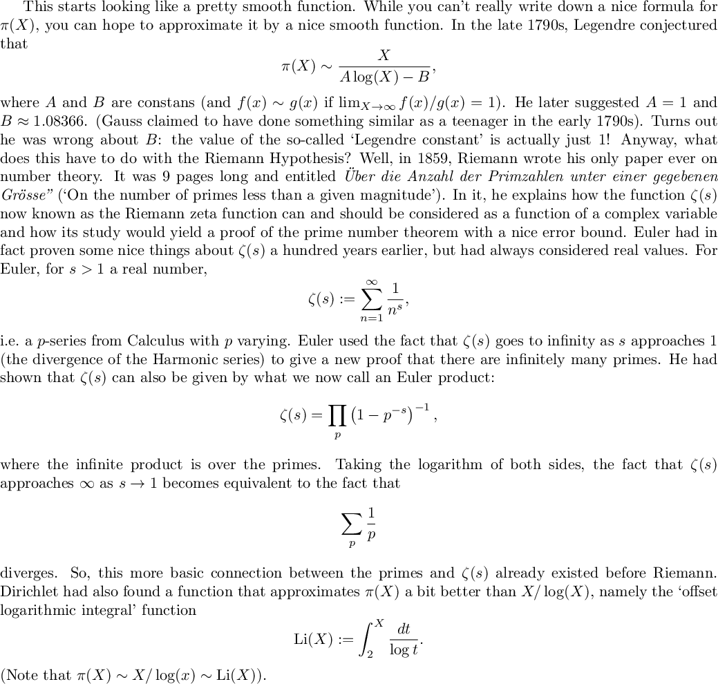
%latex
This starts looking like a pretty smooth function. While you can't really write down a nice formula for $\pi(X)$, you can hope to approximate it by a nice smooth function. In the late 1790s, Legendre conjectured that
\[
    \pi(X)\sim\frac{X}{A\log(X)-B},
\]
where $A$ and $B$ are constans (and $f(x)\sim g(x)$ if $\lim_{X\rightarrow\infty}f(x)/g(x)=1$). He later suggested $A=1$ and $B\approx1.08366$. (Gauss claimed to have done something similar as a teenager in the early 1790s). Turns out he was wrong about $B$: the value of the so-called `Legendre constant' is actually just $1$! Anyway, what does this have to do with the Riemann Hypothesis? Well, in 1859, Riemann wrote his only paper ever on number theory. It was 9 pages long and entitled \textit{\"Uber die Anzahl der Primzahlen unter einer gegebenen Gr\"osse''} (`On the number of primes less than a given magnitude'). In it, he explains how the function $\zeta(s)$ now known as the Riemann zeta function can and should be considered as a function of a complex variable and how its study would yield a proof of the prime number theorem with a nice error bound. Euler had in fact proven some nice things about $\zeta(s)$ a hundred years earlier, but had always considered real values. For Euler, for $s>1$ a real number,
\[
    \zeta(s):=\sum_{n=1}^\infty\frac{1}{n^s},
\]
i.e.\ a $p$-series from Calculus with $p$ varying. Euler used the fact that $\zeta(s)$ goes to infinity as $s$ approaches $1$ (the divergence of the Harmonic series) to give a new proof that there are infinitely many primes. He had shown that $\zeta(s)$ can also be given by what we now call an Euler product:
\[
    \zeta(s)=\prod_p\left(1-p^{-s}\right)^{-1},
\]
where the infinite product is over the primes. Taking the logarithm of both sides, the fact that $\zeta(s)$ approaches $\infty$ as $s\rightarrow1$ becomes equivalent to the fact that
\[
    \sum_p\frac{1}{p}
\]
diverges. So, this more basic connection between the primes and $\zeta(s)$ already existed before Riemann. Dirichlet had also found a function that approximates $\pi(X)$ a bit better than $X/\log(X)$, namely the `offset logarithmic integral' function
\[
    \operatorname{Li}(X):=\int_2^X\frac{dt}{\log t}.
\]
(Note that $\pi(X)\sim X/\log(x)\sim\operatorname{Li}(X)$).

P = plot(prime_pi(x), (x,2,10^3), legend_label='$\pi(X)$', legend_color='blue') + plot(Li(x),(x,2,10^3), color='red', legend_label='$Li(X)$', legend_color='red') + plot(x/log(x), (x, 2, 10^3), color='green', legend_label='$x/\log(x)$', legend_color='green')
P.show(legend_loc='right')
P.save("Approx_10_3.pdf", legend_loc='right')
P = plot(prime_pi(x), (x,2,10^6), legend_label='$\pi(X)$', legend_color='blue') + plot(Li(x),(x,2,10^6), color='red', legend_label='$Li(X)$', legend_color='red') + plot(x/log(x), (x, 2, 10^6), color='green', legend_label='$x/\log(x)$', legend_color='green')
P.show(legend_loc='right')
P.save("Approx_10_6.pdf", legend_loc='right')

plot(prime_pi(x) / x, (x,2,10^3))
plot(prime_pi(x) / x, (x,2,10^6))

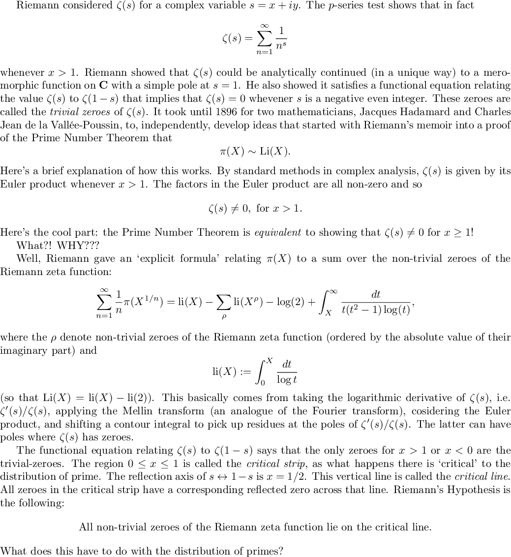
%latex
Riemann considered $\zeta(s)$ for a complex variable $s=x+iy$. The $p$-series test shows that in fact
\[
    \zeta(s)=\sum_{n=1}^\infty\frac{1}{n^s}
\]
whenever $x>1$. Riemann showed that $\zeta(s)$ could be analytically continued (in a unique way) to a meromorphic function on $\mathbf{C}$ with a simple pole at $s=1$. He also showed it satisfies a functional equation relating the value $\zeta(s)$ to $\zeta(1-s)$ that implies that $\zeta(s)=0$ whevener $s$ is a negative even integer. These zeroes are called the \textit{trivial zeroes} of $\zeta(s)$. It took until 1896 for two mathematicians, Jacques Hadamard and Charles Jean de la Vall\'ee-Poussin, to, independently, develop ideas that started with Riemann's memoir into a proof of the Prime Number Theorem that
\[
    \pi(X)\sim\operatorname{Li}(X).
\]
Here's a brief explanation of how this works. By standard methods in complex analysis, $\zeta(s)$ is given by its Euler product whenever $x>1$. The factors in the Euler product are all non-zero and so
\[
    \zeta(s)\neq0,\text{ for }x>1.
\]
Here's the cool part: the Prime Number Theorem is \textit{equivalent} to showing that $\zeta(s)\neq0$ for $x\geq1$!

What?! WHY???

Well, Riemann gave an `explicit formula' relating $\pi(X)$ to a sum over the non-trivial zeroes of the Riemann zeta function:
\[
\sum_{n=1}^\infty\frac{1}{n}\pi(X^{1/n})=\operatorname{li}(X)-\sum_\rho\operatorname{li}(X^\rho)-\log(2)+\int_X^\infty\frac{dt}{t(t^2-1)\log(t)},
\]
where the $\rho$ denote non-trivial zeroes of the Riemann zeta function (ordered by the absolute value of their imaginary part) and
\[\operatorname{li}(X):=\int_0^X\frac{dt}{\log t}
\](so that $\operatorname{Li}(X)=\operatorname{li}(X)-\operatorname{li}(2)$).
This basically comes from taking the logarithmic derivative of $\zeta(s)$, i.e.\ $\zeta^\prime(s)/\zeta(s)$, applying the Mellin transform (an analogue of the Fourier transform), cosidering the Euler product, and shifting a contour integral to pick up residues at the poles of $\zeta^\prime(s)/\zeta(s)$. The latter can have poles where $\zeta(s)$ has zeroes.

The functional equation relating $\zeta(s)$ to $\zeta(1-s)$ says that the only zeroes for $x>1$ or $x<0$ are the trivial-zeroes. The region $0\leq x\leq1$ is called the \textit{critical strip}, as what happens there is `critical' to the distribution of prime. The reflection axis of $s\leftrightarrow1-s$ is $x=1/2$. This vertical line is called the \textit{critical line}. All zeroes in the critical strip have a corresponding reflected zero across that line. Riemann's Hypothesis is the following:
\[
    \text{All non-trivial zeroes of the Riemann zeta function lie on the critical line.}
\]
What does this have to do with the distribution of primes?

#Error term in the Prime Number Theorem
plot(Li(x)-prime_pi(x), (x,2,10^6)) + plot(sqrt(x)*log(x) / 130,(x,2,10^6),color='red')

%latex
The Riemann Hypothesis tells you about how well $\operatorname{Li}(X)$ approximates $\pi(X)$. In the so-called explicit formula mentioned above, estimating the sum over non-trivial zeroes of the Riemann zeta function gives an estimate of the error in the approximation $\pi(X)\approx\operatorname{Li}(x)$. So, while proving the Prime Number Theorem involves showing the zero-free region of $\zeta(s)$ can be extended from $x>1$ to $x\geq1$, pushing the zero-free region further left improves the error estimate. In fact, the supremum of the real part of the non-trivial zeroes of $\zeta(s)$ equals the infimum of the numbers $r$ such that
\[
    \mid\pi(X)-\operatorname{Li}(X)\mid=O(X^r).
\]
As such, the Riemann Hypothesis ensures the optimal bound on the error in the Prime Number Theorem: if RH holds, then
\[
    \mid\pi(X)-\operatorname{Li}(X)\mid=O(X^{1/2}\log(X)).
\]

%latex
It's known that at least 40\% of non-trivial zeroes lie on the critical line. It has been computationally verified that the first $10^{13}$ non-trivial zeroes all lie on the critical line. This is a lot! So, why isn't it enough to know that?

plot(li(x)-prime_pi(x), (x,2,10^9))

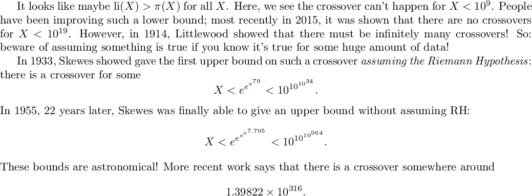
%latex
It looks like maybe $\operatorname{li}(X)>\pi(X)$ for all $X$. Here, we see the crossover can't happen for $X<10^9$. People have been improving such a lower bound; most recently in 2015, it was shown that there are no crossovers for $X<10^{19}$. However, in 1914, Littlewood showed that there must be infinitely many crossovers! So: beware of assuming something is true if you know it's true for some huge amount of data!

In 1933, Skewes showed gave the first upper bound on such a crossover \textit{assuming the Riemann Hypothesis}: there is a crossover for some
\[
    X<e^{e^{e^{79}}}<10^{10^{10^{34}}}.
\]
In 1955, 22 years later, Skewes was finally able to give an upper bound without assuming RH:
\[
    X<e^{e^{e^{e^{7.705}}}}<10^{10^{10^{964}}}.
\]
These bounds are astronomical! More recent work says that there is a crossover somewhere around
\[1.39822\times10^{316}.\]