3. Propagation of Uncertainty

3.1 Introduction

Suppose that you've measured quantities $a$, $b$, $c$, … with uncertainties $U_a$, $U_b$, $U_c$, …, and you are calculating a function $f(a,b,c,\ldots)$. For example, you might calculate the average speed of an object by dividing the distance covered by the time elapsed. How would you find the uncertainty of the average speed from the uncertainties of the distance and time? The general process of finding the uncertainty of a calculated quantity is called the propagation of uncertainty.

3.2 General Method

If quantity $a$ varies by $U_a$ while $b$, $c$, … are held constant, then the function $f(a,b,c,\ldots)$ will vary by $(\partial f/\partial a)U_a$. There are similar variations in $f$ when the other variables are varied individually. If variations in $f$ due to each of the quantitiess are independent of each other, the uncertainty of $f$ due to the uncertainties of all of the quantities is

In other words, the variations due to each variable combine like the components of a vector do to give the length of the vector. Note that this is based on the assumption that the variations in $a$, $b$, ... are independent of each other.

3.3 Two Frequently-Used Examples

3.3.1 Addition or Subtraction

If the function is a sum or difference, $f = a \pm b$, then the partial derivatives are $\partial f/\partial a = 1$ and $\partial f/\partial a = \pm 1$. Using equation 3.1, the uncertainty in $f$ is

for both addition and subtraction.

If $f = a + b + \ldots - c - d - \ldots$, then equation 3.2 generalizes to

3.3.2 Multiplication or Division

If the function is $f = ab$, then $\partial f/\partial a = b$ and $\partial f/\partial b = a$. Using equation 3.1, the uncertainty in $f$ is

This can be rewritten as

or

The same result holds for division (see problem 3.1). The uncertainty of a quantity divided by that quantity ($U_a/a$, for example) is called a fractional uncertainty. For multiplication or division, the fractional uncertainties combine the same way as uncertainties commbine for addition or subtraction. Note that equations 3.5 and 3.6 cannot be used to calculate the uncertainty of $a^2$ by setting $a = b$ (see problem 3.2).

If $f = (ab\cdots)/(cd\cdots)$, then equation 3.6 generalizes to

3.4 Examples

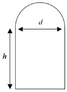
Example 3.1: Suppose that you measure the dimensions of the object below as $D = 4.24 \pm 0.03 \ \rm{cm}$ and $H = 6.07 \pm 0.04 \ \rm{cm}$.

Are your measurements consistent with those of someone who reports $A = 31.32 \pm 0.61 \ \rm{cm^2}$?

In the intermediate steps, we'll keep several digits and display the appropriate number of significant figures in the final step. The area in terms of the measured dimensions $D$ and $H$ is

which gives

Using equation 3.1, the uncertainty of the area is

which gives

Rounding the uncertainty to two significant figures and the area to the same decimal place, the measured area is $32.80 \pm 0.33\ \rm{cm}^2$. The expected ranges for the area are $32.47 - 33.13\ \rm{cm}^2$ and $30.71 - 31.93\ \rm{cm}^2$, which do not overlap, so they are not consistent.

Example 3.2: Suppose that the number of bacteria in a certain colony at a certain time is $N = 40,000 \pm 200$. What is $f = \ln N$? Your answer should include an uncertainty.

The value of $f$ is $\ln(40,000) = 10.5966$. The partial derivative of $f$ with respect to $N$ is $\partial f/\partial N = 1/N$, so

Rounding $\ln N$ to the same decimal place as the uncertainty, the anwser is $10.597 \pm 0.005$.

3.5 Uncertainty Calculations Using Python

You should learn how to perform uncertainty calculations by hand. Once you've done that, you may also use the uncertainties package in Python. This is described in one of the Computation Tutorials.

3.6 Problems

3.1 Show that equation 3.6 also holds for $f = a/b$.

3.2 Equations 3.5 and 3.6 cannot be used to calculate the uncertainty of $a^2$ by setting $a = b$.    (a) Explain why those equations can't be used to find $U_{a^2}$.    (b) Using equation 3.1, find the correct expression for $U_{a^2}$.

3.3 Find an expression for the uncertainty of $f = A \cos (Bx)$, where $A$ and $B$ are constants.

3.4 Suppose that $x$ is measured to be $85 \pm 3$. What are the value and uncertainty of $\log_{10} x$? It will be helpful to know that $$\frac{d}{dx}(\log_{10} x) = \frac{1}{x \ln 10}.$$

3.5 Suppose that a sample of water with a mass of 1.5 ± 0.1 kg starts at a temperature of 275 ± 4 K and finishes at a temperature of 331 ± 2 K. The specific heat of water is $c$ = 4186 J/(kg K) with negligible uncertainty. The amount of energy that must flow into the water to cause this temperature increase is given by $Q = mc\Delta T$, where $\Delta T = T_f - T_i$ is the change in temperature. Find the heat flow and its uncertainty. (Hint: First, find $\Delta T$ and it uncertainty. Treat $\Delta T$ as a single variable for the final part of the calculation.)