%latex
\section*{The Birch and Swinnerton-Dyer Conjecture}
In the talk last Thursday, Joe Silverman told his about taxicab numbers and elliptic curves. So, the first Millenium Problem I'll tell you about is the one about elliptic curves: the Birch and Swinnerton-Dyer Conjecture.

This conjecture, commonly known as BSD, is about the rational points on an elliptic curve defined over $\mathbf{Q}$. An \textit{elliptic curve} is a curve $E$ in the $xy$-plane defined by an equation of the form
\[
    E:y^2=x^3+Ax+B,
\]
where we require the cubic polynomial on the right-hand side to have distinct roots (so that the curve is `smooth'). Recall also that we think of there being a point $\infty$ out at infinity, as well.

We say that the curve is \textit{defined over $\mathbf{Q}$} if $A,B\in\mathbf{Q}$ (and there is a point on the curve with rational coordinates, though in this form that point is simply $\infty$). The \textit{group of rational points on $E$} (aka the \textit{Mordell--Weil group of $E$}) is
\[
    E(\mathbf{Q}):=\{\text{points $(x,y)$ on $E$ such that }x,y\in\QQ\}\cup\{\infty\}.
\]
One amazing thing Joe Silverman told us about is that if you have two points in $E(\mathbf{Q})$, then you can `add' them to get a third point and this makes $E(\mathbf{Q})$ into an abelian group. In 1922, Mordell proved the foundational result that $E(\mathbf{Q})$ is a \textit{finitely-generated} abelian group. Specifically, this means that
\[
    E(\mathbf{Q})\cong(\text{finite group})\times\mathbf{Z}^{r(E)},
\]
where $r(E)$ is a non-negative integer called the \textit{rank of $E$}. The finite groups that appear are well-understood. Indeed, in 1977, Barry Mazur proved that there are exactly 15 possibilites for it:
\[
    \mathbf{Z}/N\mathbf{Z},\text{ for }N=1,2,\dots,10,\text{ or }12
\]
or
\[
    \mathbf{Z}/2\mathbf{Z}\times\mathbf{Z}/2N\mathbf{Z},\text{ for }N=1,2,3,\text{ or }4.
\]
Furthermore, there are efficient algorithms for computing the so-called `torsion subgroup' of an elliptic curve. The rank is much more mysterious. It is conjectured that it can be arbitrarily large, but the record is held by Noam Elkies for a curve of rank at least 28. On the other hand, it is conjectured that 50\% of curves have rank $0$ and 50\% have rank 1, but it's only in the last five years, with the work of Manjul Bhargava and Arul Shankar that the average rank has been shown to be finite. Furthermore, there aren't efficient algorithms for computing the rank.

The BSD conjecture is basically about determining the rank of an elliptic curve over $\mathbf{Q}$ in terms of the number of solutions to $y^2=x^3+Ax+B$ modulo primes.

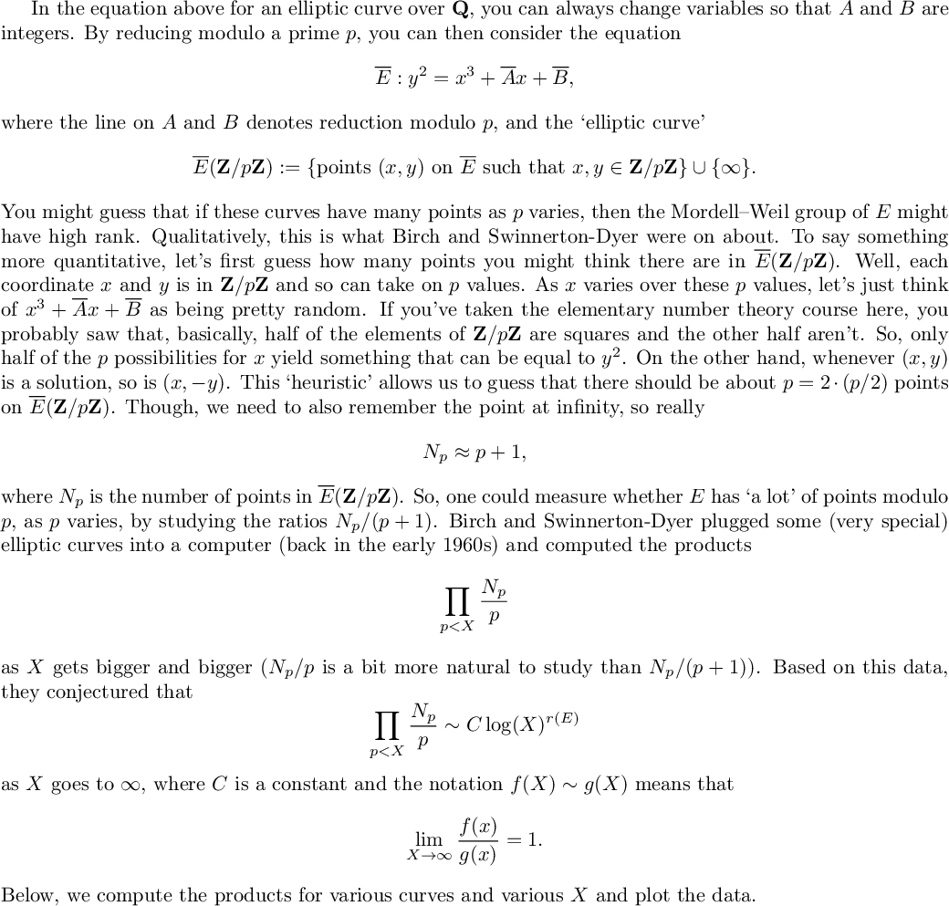
%latex
In the equation above for an elliptic curve over $\mathbf{Q}$, you can always change variables so that $A$ and $B$ are integers. By reducing modulo a prime $p$, you can then consider the equation
\[
\overline{E}:y^2=x^3+\overline{A}x+\overline{B},
\]where the line on $A$ and $B$ denotes reduction modulo $p$, and the `elliptic curve'
\[
    \overline{E}(\mathbf{Z}/p\mathbf{Z}):=\{\text{points $(x,y)$ on $\overline{E}$ such that }x,y\in\mathbf{Z}/p\mathbf{Z}\}\cup\{\infty\}.
\]
You might guess that if these curves have many points as $p$ varies, then the Mordell--Weil group of $E$ might have high rank. Qualitatively, this is what Birch and Swinnerton-Dyer were on about. To say something more quantitative, let's first guess how many points you might think there are in $\overline{E}(\mathbf{Z}/p\mathbf{Z})$. Well, each coordinate $x$ and $y$ is in $\mathbf{Z}/p\mathbf{Z}$ and so can take on $p$ values. As $x$ varies over these $p$ values, let's just think of $x^3+\overline{A}x+\overline{B}$ as being pretty random. If you've taken the elementary number theory course here, you probably saw that, basically, half of the elements of $\mathbf{Z}/p\mathbf{Z}$ are squares and the other half aren't. So, only half of the $p$ possibilities for $x$ yield something that can be equal to $y^2$. On the other hand, whenever $(x,y)$ is a solution, so is $(x,-y)$. This `heuristic' allows us to guess that there should be about $p=2\cdot(p/2)$ points on $\overline{E}(\mathbf{Z}/p\mathbf{Z})$. Though, we need to also remember the point at infinity, so really
\[
    N_p\approx p+1,
\]
where $N_p$ is the number of points in $\overline{E}(\mathbf{Z}/p\mathbf{Z})$. So, one could measure whether $E$ has `a lot' of points modulo $p$, as $p$ varies, by studying the ratios $N_p/(p+1)$. Birch and Swinnerton-Dyer plugged some (very special) elliptic curves into a computer (back in the early 1960s) and computed the products
\[
    \prod_{p<X}\frac{N_p}{p}
\]
as $X$ gets bigger and bigger ($N_p/p$ is a bit more natural to study than $N_p/(p+1)$). Based on this data, they conjectured that
\[
    \prod_{p<X}\frac{N_p}{p}\sim C\log(X)^{r(E)}
\]
as $X$ goes to $\infty$, where $C$ is a constant and the notation $f(X)\sim g(X)$ means that
\[
    \lim_{X\rightarrow\infty}\frac{f(x)}{g(x)}=1.
\]
Below, we compute the products for various curves and various $X$ and plot the data.

#Cremona's database of elliptic curves (ordered by 'conductor')
CD = CremonaDatabase(set_global=True)

#An iterator for the curves of conductor < 100
CDiter = CD.iter(range(100))

#The first curve in the database
E = CDiter.next()
E

E.rank()
E.torsion_subgroup()

X = 10^6 #bound on the primes
prime_pi(10^6) #number of primes

number_of_bins = 1000

import sys #For forcing sage to print to screen at certain points

#Computing the product for number_of_bins many values of X
bin_width = X / number_of_bins
current_bin = bin_width
products = [[current_bin, 1]]
for p in prime_range(X+1):
    if p > current_bin:
        current_bin += bin_width
        products.append([current_bin, products[-1][1]])
        if len(products) % 50 == 0:
            print len(products)
            sys.stdout.flush()
    products[-1][-1] *= (E.Np(p) / p).n()

#Plot of the product up to X versus X
list_plot(products)

#The above graph is pretty much "constant", right?

#Find a curve of positive rank
while E.rank() == 0:
    E = CDiter.next()
E

#The equation for E in the form given above
E.short_weierstrass_model()

E.rank()

#I've basically copy-pasted the code above here to just make it a function we can call
def Np_product(E, X=10^6, number_of_bins=1000): #This function takes one input, E, and two optional inputs, X and number_of_bins
    bin_width = X / number_of_bins
    current_bin = bin_width
    products = [[current_bin, 1]]
    for p in prime_range(X+1):
        if p > current_bin:
            current_bin += bin_width
            products.append([current_bin, products[-1][1]])
            if len(products) % 50 == 0:
                print len(products)
                sys.stdout.flush()
        products[-1][-1] *= (E.Np(p) / p)
    return products

#Computing the product for number_of_bins many values of X
products1 = Np_product(E)

list_plot(products1)

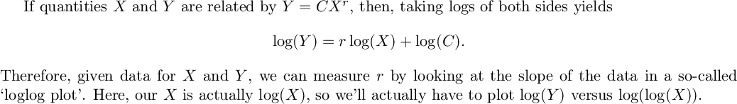
#This does *not* look constant
︠aaa9b103-0d97-4477-8ead-3302d7510e92︠
%latex
If quantities $X$ and $Y$ are related by $Y=CX^r$, then, taking logs of both sides yields
\[
    \log(Y)=r\log(X)+\log(C).
\]
Therefore, given data for $X$ and $Y$, we can measure $r$ by looking at the slope of the data in a so-called `loglog plot'. Here, our $X$ is actually $\log(X)$, so we'll actually have to plot $\log(Y)$ versus $\log(\log(X))$.

products1_log = [[x.n().log().log(), y.n().log()] for x, y in products1]

#A logloglogplot
P1 = list_plot(products1_log)
P1.show()

#We can find a linear fit to this data
var('m', 'b')
mymodel(x) = m * x + b
myfit = find_fit(products1_log, mymodel, solution_dict=True)

myfit[m] # "Almost" 1!

(P1 + plot(myfit[m] * x + myfit[b], (x,1.7,2.7), color='red')).show()

#Find a curve of rank 2
for E in CD.iter([389]):
    if E.rank() == 2:
        break
E

products2 = Np_product(E)

products2_log = [[x.n().log().log(), y.n().log()] for x, y in products2]

P2 = list_plot(products2_log)
P2.show()

#Not constant again. Does it look like Clog(X)^2?
︠c165ffb1-a222-4f86-a6b8-4d2383642062︠
myfit2 = find_fit(products2_log, mymodel, solution_dict=True)

myfit2[m] # "Just about" 2!

var('x')
(P2 + plot(myfit2[m] * x + myfit2[b], (x,1.7,2.7), color='red')).show()

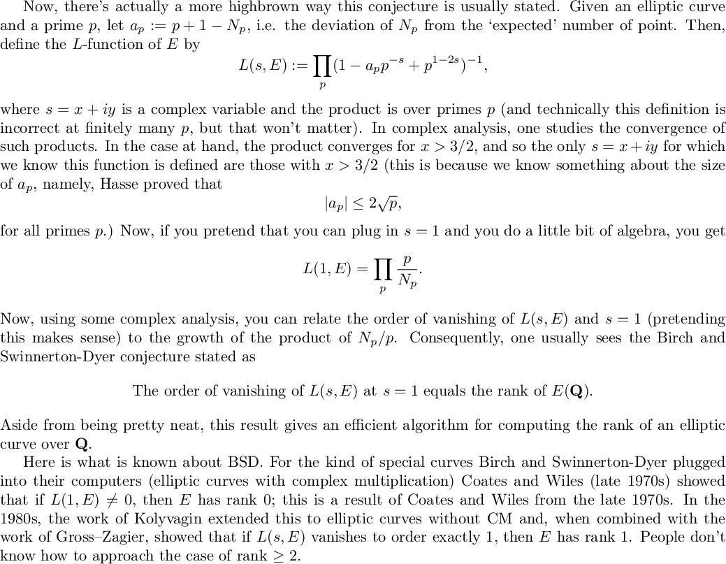
%latex
Now, there's actually a more highbrown way this conjecture is usually stated. Given an elliptic curve and a prime $p$, let $a_p:=p+1-N_p$, i.e. the deviation of $N_p$ from the `expected' number of point. Then, define the $L$-function of $E$ by
\[
    L(s,E):=\prod_p(1-a_pp^{-s}+p^{1-2s})^{-1},
\]
where $s=x+iy$ is a complex variable and the product is over primes $p$ (and technically this definition is incorrect at finitely many $p$, but that won't matter). In complex analysis, one studies the convergence of such products. In the case at hand, the product converges for $x>3/2$, and so the only $s=x+iy$ for which we know this function is defined are those with $x>3/2$ (this is because we know something about the size of $a_p$, namely, Hasse proved that
\[
    |a_p|\leq2\sqrt{p},
\]
for all primes $p$.) Now, if you pretend that you can plug in $s=1$ and you do a little bit of algebra, you get
\[
    L(1,E)=\prod_p\frac{p}{N_p}.
\]
Now, using some complex analysis, you can relate the order of vanishing of $L(s,E)$ and $s=1$ (pretending this makes sense) to the growth of the product of $N_p/p$. Consequently, one usually sees the Birch and Swinnerton-Dyer conjecture stated as
\[
    \text{The order of vanishing of $L(s,E)$ at $s=1$ equals the rank of $E(\mathbf{Q})$}.
\]
Aside from being pretty neat, this result gives an efficient algorithm for computing the rank of an elliptic curve over $\mathbf{Q}$.

Here is what is known about BSD. For the kind of special curves Birch and Swinnerton-Dyer plugged into their computers (elliptic curves with complex multiplication) Coates and Wiles (late 1970s) showed that if $L(1,E)\neq0$, then $E$ has rank $0$; this is a result of Coates and Wiles from the late 1970s. In the 1980s, the work of Kolyvagin extended this to elliptic curves without CM and, when combined with the work of Gross--Zagier, showed that if $L(s,E)$ vanishes to order exactly 1, then $E$ has rank $1$. People don't know how to approach the case of rank $\geq2$.