Jack Montoro

K-Means Clustering Final Project Lecture

Math 157

Monday, March 20, 2023

Run this first

K-means clustering is an algorithm that takes in a data point value and evaluates its category on a basis not dissimilar to the K-Nearest Neighbors algorithm, but instead of looking for individual data points as neighbors, it looks for clusters as neighbors. We will review KNN below and later take a look at K-means clusters.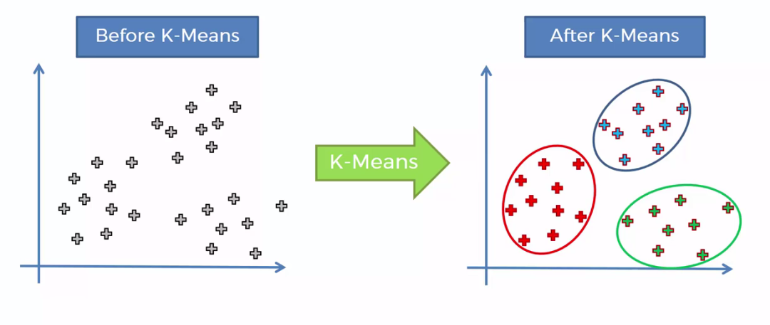

K Nearest Neighbor Review:

K Nearest Neighbors is a supervised machine learning algorithm that we may use for regression or classification tasks. The inherent advantage of the KNN algorithm is that we do not need to make assumptions about the distributions of the data we are analyzing.

However, we do assume similarities between existing case data that we have access to and new data collected in order to group the new data. We group this new data according to its proximity to categories we have formed for the existing cases. For example, in the following photo we evaluate the new datum according to the classes A and B that we have established from the existing data. We evaluate the new datum on the basis of its proximity to the other entries, and assign its category.

In the previous example we we looking at the 3 neighbor points closest to our new entry to classify the node, so we can deduce that k=3 here. How we define "proximity" is up to the implementation method of the data analyst, but one potential method of calculating proximity is the euclidean distance formula.

Once we have the count of the categories of the k nearest neighbors, we can assign a category to our newest entry depending on which category among the k neighbors had the greatest count.

This same distance formula will later be used to calculate the distances between our points for k-means clusters.

If we decide to go with euclidean distance formula as our distance function, we can calculate via $\sqrt{\sum_{i=1}^{n} (q_{i} - p_{i})^{2}} = \sqrt{(q_{1} - p_{1})^{2} + (q_{2} - p{2})^{2} + ... + (q_{n} - p_{n})^{2}}$ where p and q are separate points of dimension $n$. The following example is the trivial n=2:

Participation Check:

In the cell below, implement a function that returns the Euclidean distance of two points in dimension 2:

Here, we will use the iris dataset to build a dataframe and demonstrate our algorithm.

Here we obtain a new DataFrame X, which is iris, but with only the 4 relevant categories that we will use for our distance formula.

Once we have chosen our distance function, we can calculate the distance from our test data point to each of the other points in our dataset. Once we have calculated these values in the form of an array, we can sort the array to get the data points in terms of their distance to our test value.

We can then use the most common label of the k nearest points in the distance array, to find the category of our test point. We repeat this process until we have categorized all of our test points.

Of our 10 nearest neighbors, we can see that Iris-setosa is the most frequent species category the appears, so we would assign our test value this species label.

K-Means Clustering Algorithm

This method that we use in KNN algorithm for data point categorization is utilized in k-means where we do not need to assume we have any information about species, but categorize the information according to selected cluster values, and each cluster is defined by our given distance formula.

We select k clusters for which we calculate k means. Selecting the optimal k value can be achieved by iterating over each value of k to k = n (where n is the number of data entries) and plotting the variance of the clusters against each value of k.

To get the optimal value of k, we find the value of k after which the rate of variance reduction diminishes.

In this example, the optimal k value would be 2, as we can observe above that the rate of variation decrease between clusters drops of at 2 clusters.

Below, we obtains the optimal cluster set for the collected data when k=3.

We typically get a cluster by choosing three points at random, and designating them as our cluster points.

We then form our clusters by calculating the distance of each point to each of the three clusters. We assign each point to the cluster it is closest to.

Once every point is assigned, we get the mean of each cluster, and calculate the clusters again by assigning each point its cluster by calculating its proximity to this calculated mean.

We repeat this last process until the means of clusters calculated from our latest iteration is the same as the means calculated from our previous iteration.

This is a lot of work, but thankfully with the Julia package Clusters, we can calculate the k-means for our data with just a single function.

We can see from the plot that our "elbow" value is k=3, as this is the point where the rate of decrease for SSE per k value falls off.

We know this is the case as there are in fact three species of iris, but we can verify visually with scatter plots that this is true.

In the plots above, we can see that variation between the point clusters drops off most precipitously when k=3. This means that adding more clusters has diminishing returns for the distance of each data point to its cluster mean as visualized in the SSE plot. This means that adding more clusters will probably not provide greater optimization of our categories. Therefore, we may conclude that k=3 is the optimal categorization.

K-means Clustering may be applied to a plethora of real-world examples, such as targeted ad campaigns that group customers according to available data to determine potential interest in a product or service It may also be used to detect patterns in fraud, data breaches, or IT alerts based on observed commonalities between incidents.

Homework Questions:

Problem 1) Alternative distance formula:

You may run into situations where you would like to use some formula other than Euclidean distance to calculate the distance between datapoints. One alternative you may choose is the Minkowski Distance Formula.

This formula is represented as

where n is the dimensions of the data points, x is your first point, y is your second point, and p is the power parameter. For instance, if your power parameter is 2, your distance is Euclidean.

Using the kmeans function, find a k value that optimizes the kmeans clusters for the following dataset:

We notice that the row number is equal to the SI number and Customer Key is an arbitrary value, so this column is superfluous. We can clean up the data further:

For this dataframe, utilize the kmeans function to get the best approximate categorization of clusters

Part 1: Arrange the Dataframe "credit" so we can get k-means for a k-value of 2.

Part 2: Write a function to return a vector of size 10 filled with all the kmeans objects for our given data from k=1 to k=10.

Part 3: Plot your information with the k-values in the X-axis and the SSE for each k-value in the Y-axis.

Solutions:

Participation Check Euclidean Distance:

Minkowski Distance Solution:

K-Means For Credit Card Data Solution

We can see that the "elbow" point on this plot is k=3, so we can conclude that the optimal number of k-means clusers is 3.

We verify the results below.